
Variational autoencoder on the CIFAR-10 dataset 1.
- 11 minsVariational autoencoder - VAE
I just recently got familiar with this concept and the underlying theory behind it thanks to the CSNL group at the Wigner Institute. This happenes to be the most amazing thing I have occupied with so far in this field and I hope you, My reader, will enjoy going through this article.
I am going to use the CIFAR-10 dataset through-out this article and provide examples and useful explanations while going to the method and building a variational autoencoder with Tensorflow. The article I used was this one written by Kingma and Welling. The excersice code to study and try to use all this can be found on GitHub thanks to David Nagy.
import tensorflow as tf
import numpy as np
import matplotlib.pyplot as plt
# Importing the dataset
from tensorflow.keras.datasets.cifar10 import load_data
(X_train, y_train), (X_test, y_test) = load_data()
X_train.shape, y_train.shape, X_test.shape, y_test.shape
((50000, 32, 32, 3), (50000, 1), (10000, 32, 32, 3), (10000, 1))
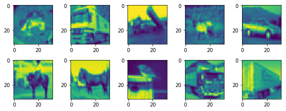
# Plot the first ten images
n_images = 10

import matplotlib.pyplot as plt
import matplotlib.image as mpimg

def rgb2gray(rgb):
    return np.dot(rgb[...,:3], [0.299, 0.587, 0.114])

X_train = rgb2gray(X_train)

plt.figure(figsize=(n_images + 6, 6))
for i in range(n_images // 2):
    plt.subplot(4, n_images, i+1)
    plt.imshow(X_train[i])
    plt.subplot(4, n_images, n_images+i+1)
    plt.imshow(X_train[n_images+i+1])
plt.tight_layout()
# Usually is it set to be a multiple of two (computational reason)
batch_size = 1000

n_h1 = 1024
n_h2 = 512
latent_dim = 15

# Placeholder for the flattened input image
x = tf.placeholder(dtype=tf.float32, shape=(None, 32*32))

# Weights and biases for the ENCODER

"""
    ENCODER
"""

# First hidden layer
W1 = tf.Variable(tf.truncated_normal(shape=(32*32, n_h1), stddev=0.1))
b1 = tf.Variable(tf.truncated_normal(stddev=0.01, shape=[n_h1]))
h1 = tf.nn.sigmoid(tf.add(tf.matmul(x, W1), b1))

# Second hidden layer
W2 = tf.Variable(tf.truncated_normal(shape=(n_h1, n_h2), stddev=0.1))
b2 = tf.Variable(tf.truncated_normal(stddev=0.01, shape=[n_h2]))
h2 = tf.nn.sigmoid(tf.add(tf.matmul(h1, W2), b2))

# /assets/images/20190222/output weights and biases to latent space
W3_mean = tf.Variable(tf.truncated_normal(shape=(n_h2, latent_dim), stddev=0.1))
b3_mean = tf.Variable(tf.truncated_normal(stddev=0.01, shape=[latent_dim]))

W3_var = tf.Variable(tf.truncated_normal(shape=(n_h2, latent_dim), stddev=0.1))
b3_var = tf.Variable(tf.truncated_normal(stddev=0.01, shape=[latent_dim]))

mean = tf.add(tf.matmul(h2, W3_mean), b3_mean)
var = tf.add(tf.matmul(h2, W3_var), b3_var)
In the article a reparametrization trick is used to make the cost optimization computationally feasible. Therefore z - the latent variable is written as follows:
# For computational reasons as well
eps = tf.random_normal(shape=(batch_size, latent_dim))
z = mean + tf.multiply(tf.sqrt(tf.exp(var)), eps)
n_h1_ = 256
n_h2_ = 512

# Weights and biases for the DECODER

"""
    DECODER
    same structure as the ENCODER with different layer sizes
"""

W1_ = tf.Variable(tf.truncated_normal(shape=(latent_dim, n_h1_), stddev=0.01))
b1_ = tf.Variable(tf.truncated_normal(stddev=0.01, shape=[n_h1_]))
h1_ = tf.nn.sigmoid(tf.add(tf.matmul(z, W1_), b1_))

W2_ = tf.Variable(tf.truncated_normal(shape=(n_h1_, n_h2_), stddev=0.01))
b2_ = tf.Variable(tf.truncated_normal(stddev=0.01, shape=[n_h2_]))
h2_ = tf.nn.sigmoid(tf.add(tf.matmul(h1_, W2_), b2_))

# /assets/images/20190222/output weights and biases to latent space
W3_ = tf.Variable(tf.truncated_normal(shape=(n_h2_, 32*32), stddev=0.01))
b3_ = tf.Variable(tf.truncated_normal(stddev=0.01, shape=[32*32]))

x_reco = tf.nn.sigmoid(tf.add(tf.matmul(h2_, W3_), b3_))
Basically Tensorflow defines a computational graph in which data can flow through easilly. These variables are going to be filled once the comp. graph is initialized and the data is provided.
The cost function consist of a recontruction term which is assumed to be a simple Bernoulli log loss while the penatly term is the Kullback-Leibler divergence which estimates how well the posterior distribution function is estimated by the prior.
The prior and posterior distibutions are assumed to be Gaussians therefore the Kullback-Leibler divergence has a closed form.
binary_cross_entropy = -tf.reduce_sum(x*tf.log(1e-10 + x_reco) + (1. - x)*tf.log(1e-10 + 1 - x_reco), 1)

kl_divergence = - 0.5 * tf.reduce_sum(1e-10 + 1 + var - tf.square(mean) - tf.exp(var), 1)

cost = tf.reduce_mean(binary_cross_entropy + kl_divergence)

optimizer = tf.train.AdamOptimizer(learning_rate=0.001).minimize(cost)
The training will run in minibatches for N epochs. The number of epochs and minibatch size are predefined. Optimaziton is done the following way.
runs = 15
n_minibatches = int(X_train.shape[0] / batch_size)

print("Number of minibatches: ", n_minibatches)

sess = tf.InteractiveSession()
init = tf.global_variables_initializer()
sess.run(init)

for epoch in range(runs):
    pbar = tf.contrib.keras.utils.Progbar(n_minibatches)
    for i in range(n_minibatches):

        x_batch = X_train[i*batch_size:(i+1)*batch_size].reshape(batch_size, 32*32)/255.
        cost_, _ = sess.run((cost, optimizer), feed_dict={x: x_batch})

        pbar.add(1,[("cost",cost_)])
Number of minibatches:  50


50/50 [==============================] - 14s 286ms/step - cost: 708.8903 - iter: 24.5000
50/50 [==============================] - 14s 282ms/step - cost: 704.7177 - iter: 24.5000
50/50 [==============================] - 15s 299ms/step - cost: 694.8706 - iter: 24.5000
50/50 [==============================] - 15s 290ms/step - cost: 691.4493 - iter: 24.5000
50/50 [==============================] - 15s 304ms/step - cost: 689.1300 - iter: 24.5000
50/50 [==============================] - 16s 329ms/step - cost: 683.2461 - iter: 24.5000
50/50 [==============================] - 15s 303ms/step - cost: 680.5180 - iter: 24.5000
50/50 [==============================] - 16s 329ms/step - cost: 679.0927 - iter: 24.5000
50/50 [==============================] - 15s 296ms/step - cost: 678.5948 - iter: 24.5000
50/50 [==============================] - 14s 285ms/step - cost: 677.8830 - iter: 24.5000
50/50 [==============================] - 14s 287ms/step - cost: 677.0237 - iter: 24.5000
50/50 [==============================] - 14s 290ms/step - cost: 676.1153 - iter: 24.5000
50/50 [==============================] - 14s 286ms/step - cost: 675.0156 - iter: 24.5000
50/50 [==============================] - 14s 284ms/step - cost: 674.6326 - iter: 24.5000
50/50 [==============================] - 14s 283ms/step - cost: 673.8401 - iter: 24.5000
It is important to normalize the data since it results in under- or overflow when it is skipped. Moving on to comparing the reconstruction with actual samples in a batch is done in the following setup:
n_rec = 10

x_batch = X_train[0:batch_size].reshape(batch_size, 32*32)/255.

plt.figure(figsize=(n_rec+2,4))
for i in range(n_rec):

    plt.subplot(4, n_rec, i+1)
    plt.imshow(x_batch[i].reshape(32, 32))

    plt.subplot(4, n_rec, n_rec+i+1)
    pred_img = sess.run(x_reco, feed_dict={x: x_batch})
    plt.imshow(pred_img[i].reshape(32, 32))

plt.tight_layout()
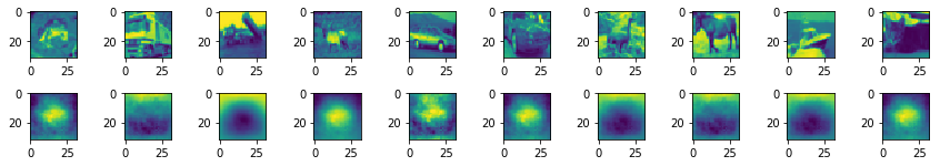
Well it can be seen that the generated images at least capture the contrast of the background correctly and some kind of shape like thing can be seen in the middle but generally nothing is familiar to the naked eye.
I’ll update this code next week with using the MNIST data set and/or changing the decoder and encoder layers to more general CNNs.
@Regards, Alex

Alex Olar
Christian, foodie, physicist, tech enthusiast