
Exploratory data analysis of streams in the USA
- 20 minsStatistical analysis of water discharge of surface streams
Large amounts of historical surface water data are available from the United States Geological Survey (USGS) at https://waterdata.usgs.gov/nwis The goal of the project is to retrieve samples from the web interface manually, and then later automate the process by calling the web service as described at https://help.waterdata.usgs.gov/faq/automated-retrievals.
Excercise 1
For the purposes of the current excercises, select a stream from a rainy area with relatively small discharge so that the effect of short but strong storms is visible. Good choices are small rivers from the north-eastern US, e.g. site 01589440. Retrieve at least 10 years of data.
import pandas as pd
from io import BytesIO
import pycurl

site_number = '01589440'
date_from = '1996-06-06'
date_to = '2006-06-06'

url = 'https://nwis.waterdata.usgs.gov/nwis/uv/?parameterCd=00060,00065&format=rdb&site_no=%s&period=&begin_date=%s\
&end_date=%s&siteStatus=all' % (site_number, date_from, date_to)

def download_data_from_url( url, savename='test.csv' ):
    '''
    One can download data with a different method that supports resume. If data is two large then it takes
    lot of time and the connection to the server might be interrupted.
    '''

    buffer = BytesIO()
    c = pycurl.Curl()
    c.setopt(c.URL, url)
    c.setopt(c.WRITEDATA, buffer)
    c.perform()
    c.close()

    body = buffer.getvalue() # Body is a byte string.
    with open( savename, 'w' ) as /assets/images/20190215/output:
        /assets/images/20190215/output.write( body.decode('utf-8')) # We have to know the encoding in order to print it to a text file

download_data_from_url(url, '%s.csv' % site_number)
data = pd.read_csv('%s.csv' % site_number, sep='\t', comment='#', skiprows=[29], parse_dates=[2])
data.head(n=10)
| agency_cd | site_no | datetime | tz_cd | 69744_00060 | 69744_00060_cd | |
|---|---|---|---|---|---|---|
| 0 | USGS | 1589440 | 1996-10-01 00:15:00 | EST | 28.0 | A:[91] |
| 1 | USGS | 1589440 | 1996-10-01 00:30:00 | EST | 28.0 | A:[91] |
| 2 | USGS | 1589440 | 1996-10-01 00:45:00 | EST | 28.0 | A:[91] |
| 3 | USGS | 1589440 | 1996-10-01 01:00:00 | EST | 28.0 | A:[91] |
| 4 | USGS | 1589440 | 1996-10-01 01:15:00 | EST | 28.0 | A:[91] |
| 5 | USGS | 1589440 | 1996-10-01 01:30:00 | EST | 28.0 | A:[91] |
| 6 | USGS | 1589440 | 1996-10-01 01:45:00 | EST | 29.0 | A:[91] |
| 7 | USGS | 1589440 | 1996-10-01 02:00:00 | EST | 29.0 | A:[91] |
| 8 | USGS | 1589440 | 1996-10-01 02:15:00 | EST | 29.0 | A:[91] |
| 9 | USGS | 1589440 | 1996-10-01 02:30:00 | EST | 29.0 | A:[91] |
Excercise 2
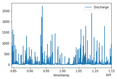
Load the downloaded data file into the processing environment paying attention to handling time stamps and perfoming the necessary data type conversions. Converting dates to floating point numbers such as unix time stamp or julian date usually makes handling time series easier. Plot the data for a certain interval to show that the effect of storms is clearly visible.
data['timestamp'] = data.datetime.map(lambda x: x.timestamp())
data.head(n=10)
| agency_cd | site_no | datetime | tz_cd | 69744_00060 | 69744_00060_cd | timestamp | |
|---|---|---|---|---|---|---|---|
| 0 | USGS | 1589440 | 1996-10-01 00:15:00 | EST | 28.0 | A:[91] | 844128900.0 |
| 1 | USGS | 1589440 | 1996-10-01 00:30:00 | EST | 28.0 | A:[91] | 844129800.0 |
| 2 | USGS | 1589440 | 1996-10-01 00:45:00 | EST | 28.0 | A:[91] | 844130700.0 |
| 3 | USGS | 1589440 | 1996-10-01 01:00:00 | EST | 28.0 | A:[91] | 844131600.0 |
| 4 | USGS | 1589440 | 1996-10-01 01:15:00 | EST | 28.0 | A:[91] | 844132500.0 |
| 5 | USGS | 1589440 | 1996-10-01 01:30:00 | EST | 28.0 | A:[91] | 844133400.0 |
| 6 | USGS | 1589440 | 1996-10-01 01:45:00 | EST | 29.0 | A:[91] | 844134300.0 |
| 7 | USGS | 1589440 | 1996-10-01 02:00:00 | EST | 29.0 | A:[91] | 844135200.0 |
| 8 | USGS | 1589440 | 1996-10-01 02:15:00 | EST | 29.0 | A:[91] | 844136100.0 |
| 9 | USGS | 1589440 | 1996-10-01 02:30:00 | EST | 29.0 | A:[91] | 844137000.0 |
data = data.rename(index=str, columns={"69744_00060": "Discharge"})
data.head(n=10)
| agency_cd | site_no | datetime | tz_cd | Discharge | 69744_00060_cd | timestamp | |
|---|---|---|---|---|---|---|---|
| 0 | USGS | 1589440 | 1996-10-01 00:15:00 | EST | 28.0 | A:[91] | 844128900.0 |
| 1 | USGS | 1589440 | 1996-10-01 00:30:00 | EST | 28.0 | A:[91] | 844129800.0 |
| 2 | USGS | 1589440 | 1996-10-01 00:45:00 | EST | 28.0 | A:[91] | 844130700.0 |
| 3 | USGS | 1589440 | 1996-10-01 01:00:00 | EST | 28.0 | A:[91] | 844131600.0 |
| 4 | USGS | 1589440 | 1996-10-01 01:15:00 | EST | 28.0 | A:[91] | 844132500.0 |
| 5 | USGS | 1589440 | 1996-10-01 01:30:00 | EST | 28.0 | A:[91] | 844133400.0 |
| 6 | USGS | 1589440 | 1996-10-01 01:45:00 | EST | 29.0 | A:[91] | 844134300.0 |
| 7 | USGS | 1589440 | 1996-10-01 02:00:00 | EST | 29.0 | A:[91] | 844135200.0 |
| 8 | USGS | 1589440 | 1996-10-01 02:15:00 | EST | 29.0 | A:[91] | 844136100.0 |
| 9 | USGS | 1589440 | 1996-10-01 02:30:00 | EST | 29.0 | A:[91] | 844137000.0 |
Excercise 3
Plot the histogram of water discharge values. Fit the data with an appropriate distribution function and bring arguments in favor of the choice of function.
from scipy.optimize import curve_fit

hist, bins = np.histogram(data['Discharge'], bins=500)

def quadratic(x, a, b, c):
    return a*x**2 + b*x + c

N = 30
# to fit the peak and a small portion of the tail after it
x = np.log(bins[:-1][:N])
y = np.log(hist[:N])

popt, pcov = curve_fit(quadratic, x, y)
perr = np.sqrt(np.diag(pcov))

print('a, b, c = ', popt)
print('err_a, err_b, err_c = ', perr)

x_test = np.linspace(0, 5, 20)
y_test = quadratic(x_test, *popt)

plt.plot(x_test, quadratic(x_test, *popt), 'r--')
plt.plot(x, y, 'o--')

plt.show()
a, b, c =  [-0.59944141  2.17443686  9.3345691 ]
err_a, err_b, err_c =  [0.03101504 0.19771276 0.30965811]
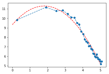
The fit is not perfect but I googled it and it was recommended on various sites that water discharge and some related geophysics phenomena should have a log normal distribution so I did fit a quadratic function on log-log scale.
data.plot('timestamp', 'Discharge')
<matplotlib.axes._subplots.AxesSubplot at 0x7fc4f1c4dcc0>
Excercise 4
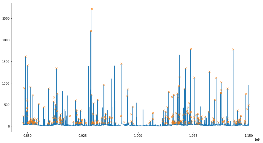
In case of small streams, storms and passing weather fronts with rain can significantly increase water discharge on a short time scale. Develop a simple algorithm to detect rainy events in the data. Plot the original time series and mark rainy events.
from scipy.signal import find_peaks
import matplotlib.pyplot as plt
import numpy as np

x = data['Discharge']
ts = data['timestamp']
peaks, _ = find_peaks(x, height=60, width=15)
plt.figure(figsize=(15, 8))
plt.plot(ts, x)
plt.plot(ts[peaks], x[peaks], "x")
plt.xticks(np.linspace(0.85e9, 1.15e9, 5))
plt.show()
Excercise 5
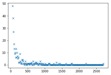
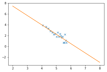
Water discharge increases significantly during rain producing maxima in the time series. Plot the distribution of maximum values and fit with an appropriate function. Bring arguments to support the choice of probabilistic model.
y_peak = x[peaks]

hist, bins = np.histogram(y_peak, bins=200)
plt.plot(bins[:-1], hist, 'x')
[<matplotlib.lines.Line2D at 0x7fc4f1c63518>]
from scipy.optimize import curve_fit

N = 19
# to exclude zeros and ones
x = np.log(bins[:-1][:N])
y = np.log(hist[:N])

def lin(x, a, b):
    return a*x + b

popt, pcov = curve_fit(lin, x, y)
perr = np.sqrt(np.diag(pcov))
print('a, b = ', popt)
print('err_a, err_b = ', perr)

plt.plot(x, y, 'x')

x_test = np.linspace(2, 8, 20)
y_test = lin(x_test, *popt)

plt.plot(x_test, y_test)
a, b =  [-1.73553201 10.93779965]
err_a, err_b =  [0.20596821 1.05340278]


[<matplotlib.lines.Line2D at 0x7fc4f1c699b0>]
Excercise 6
Once rainy events are detected, plot the distribution of the length of sunny intervals between rains. Fit the distribution with an appropriate function.
event_distance = [end_date - start_date for start_date, end_date in zip(ts[peaks], ts[peaks][1:])]

# event distance in hours instead of seconds
hist, bins = np.histogram(np.array(event_distance) / 360., bins=200)

# to exclude zeros and ones
N = 20
x = np.log(bins[:-1][:N])
y = np.log(hist[:N])

popt, pcov = curve_fit(quadratic, x, y)
perr = np.sqrt(np.diag(pcov))

print('a, b, c = ', popt)
print('err_a, err_b, err_c = ', perr)

x_test = np.linspace(0, 9, 20)
y_test = quadratic(x_test, *popt)

plt.plot(x_test, quadratic(x_test, *popt), 'r--')

plt.plot(x, y, 'o')
plt.show()
a, b, c =  [-0.13279045  0.90977024  3.029973  ]
err_a, err_b, err_c =  [0.02682844 0.2952572  0.75683953]
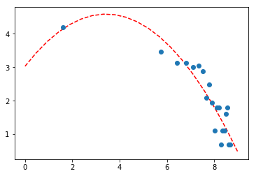
Tried to fit this with log normal as well.
Excercise 7
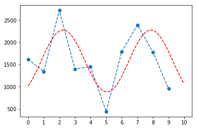
What is the maximum of water discharge in an arbitrarily chosen period of one year? Calculate the maximum of water discharge due to rain in a rolling window of 1 year, plot its distribution and fit with an appropriate function.
### fifteen minute samples one year is approx. 24*4*365 = 35040

year = 35040
maximum_dc = []
years = data['Discharge'].shape[0] // year + 1

for yr in range(0, years):
    maximum_dc.append(np.max(data['Discharge'][yr*year:(yr+1)*year]))

plt.plot(maximum_dc, 'o--')
plt.xticks(np.linspace(0, 10, 11))

def sin(x, a, b, c, d):
    return a*np.sin(b*x + c) + d

popt, pcov = curve_fit(sin, np.linspace(0, 10, 10), maximum_dc, p0=[1000, 2.*np.pi/7., 5., 1200])
perr = np.sqrt(np.diag(pcov)) 0, 100)
y_test = sin(x_test, *popt)

plt.plot(x_test, y_test, 'r--')

plt.show()
[6.97534832e+02 1.11786857e+00 5.34654194e+00 1.57949573e+03]
[2.26333346e+02 1.09895369e-01 6.38939348e-01 1.72165136e+02]
Excercise 8
How many time does it rain in a month? Calculate and plot the distribution and fit with an appropriate function.
from datetime import datetime
import collections

month = 2880
rainy_days = []
months = data['Discharge'].shape[0] // month  + 1
months_dict = dict()

for time_stamp in ts[peaks]:
    months_dict[datetime.utcfromtimestamp(int(time_stamp)).month] = 0

for time_stamp in ts[peaks]:
    months_dict[datetime.utcfromtimestamp(int(time_stamp)).month] += 1

D = collections.OrderedDict(sorted(months_dict.items()))

plt.bar(D.keys(), D.values(), align='center')
plt.show()
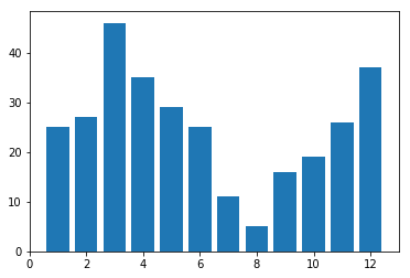
I don’t really know what kind of function fits this. It is clearly seen though that it rains the most in autumn-winter-spring and rarely in during summer.
Excercise 9
Find the measuring station you used in the excercises above on the map. Find another measurement station about 100-200 miles from it and download the data. Try to estimate the typical time it takes for weather fronts to travel the distance between the two measuring stations.
import pandas as pd

site_number = '04240010' # approx. 220 miles north - Syracuse

url = 'https://nwis.waterdata.usgs.gov/nwis/uv/?parameterCd=00060,00065&format=rdb&site_no=%s&period=&begin_date=%s\
&end_date=%s&siteStatus=all' % (site_number, date_from, date_to)

download_data_from_url(url, "%s.csv" % site_number)
data2 = pd.read_csv('%s.csv' % site_number, sep='\t', comment='#', skiprows=[32], parse_dates=[2])
data2.head(n=10)
| agency_cd | site_no | datetime | tz_cd | 107697_00060 | 107697_00060_cd | |
|---|---|---|---|---|---|---|
| 0 | USGS | 4240010 | 1996-06-06 00:00:00 | EST | 134.0 | A:[91] |
| 1 | USGS | 4240010 | 1996-06-06 00:15:00 | EST | 134.0 | A:[91] |
| 2 | USGS | 4240010 | 1996-06-06 00:30:00 | EST | 134.0 | A:[91] |
| 3 | USGS | 4240010 | 1996-06-06 00:45:00 | EST | 132.0 | A:[91] |
| 4 | USGS | 4240010 | 1996-06-06 01:00:00 | EST | 132.0 | A:[91] |
| 5 | USGS | 4240010 | 1996-06-06 01:15:00 | EST | 132.0 | A:[91] |
| 6 | USGS | 4240010 | 1996-06-06 01:30:00 | EST | 132.0 | A:[91] |
| 7 | USGS | 4240010 | 1996-06-06 01:45:00 | EST | 132.0 | A:[91] |
| 8 | USGS | 4240010 | 1996-06-06 02:00:00 | EST | 130.0 | A:[91] |
| 9 | USGS | 4240010 | 1996-06-06 02:15:00 | EST | 130.0 | A:[91] |
data2['timestamp'] = data2.datetime.map(lambda x: x.timestamp())
data2 = data2.rename(index=str, columns={"107697_00060": "Discharge"})
data2.head(n=10)
| agency_cd | site_no | datetime | tz_cd | Discharge | 107697_00060_cd | timestamp | |
|---|---|---|---|---|---|---|---|
| 0 | USGS | 4240010 | 1996-06-06 00:00:00 | EST | 134.0 | A:[91] | 834019200.0 |
| 1 | USGS | 4240010 | 1996-06-06 00:15:00 | EST | 134.0 | A:[91] | 834020100.0 |
| 2 | USGS | 4240010 | 1996-06-06 00:30:00 | EST | 134.0 | A:[91] | 834021000.0 |
| 3 | USGS | 4240010 | 1996-06-06 00:45:00 | EST | 132.0 | A:[91] | 834021900.0 |
| 4 | USGS | 4240010 | 1996-06-06 01:00:00 | EST | 132.0 | A:[91] | 834022800.0 |
| 5 | USGS | 4240010 | 1996-06-06 01:15:00 | EST | 132.0 | A:[91] | 834023700.0 |
| 6 | USGS | 4240010 | 1996-06-06 01:30:00 | EST | 132.0 | A:[91] | 834024600.0 |
| 7 | USGS | 4240010 | 1996-06-06 01:45:00 | EST | 132.0 | A:[91] | 834025500.0 |
| 8 | USGS | 4240010 | 1996-06-06 02:00:00 | EST | 130.0 | A:[91] | 834026400.0 |
| 9 | USGS | 4240010 | 1996-06-06 02:15:00 | EST | 130.0 | A:[91] | 834027300.0 |
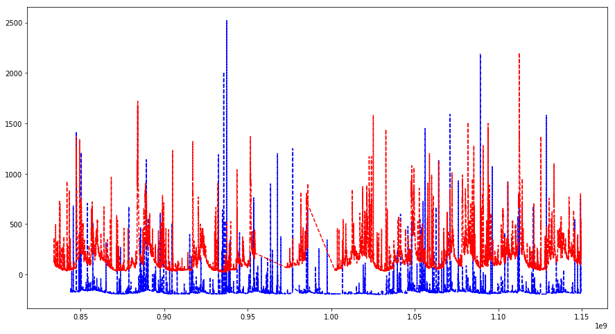
# showing it on top of each other

plt.figure(figsize=(15, 8))
plt.plot(data["timestamp"], data["Discharge"] - 200, 'b--')
plt.plot(data2["timestamp"], data2["Discharge"], 'r--')
plt.show()
# weekly rolling window 24*4*7 = 672

### fifteen minute samples one year is approx. 24*4*365 = 35040

week = 672
maximum_dc = []
maximum_dc2 = []

# assuming same number of weeks
weeks = data['Discharge'].shape[0] // week + 1

for wk in range(0, weeks):
    maximum_dc.append(np.max(data['Discharge'][wk*week:(wk+1)*week]))
    maximum_dc2.append(np.max(data2['Discharge'][wk*week:(wk+1)*week]))

plt.figure(figsize=(15, 8))

from scipy.signal import savgol_filter

plt.plot(savgol_filter(maximum_dc, 31, 2), 'b--')
plt.plot(savgol_filter(maximum_dc2, 31, 2), 'r--')
plt.xticks(np.linspace(0, 500, 26))

plt.show()
/opt/conda/lib/python3.6/site-packages/scipy/signal/_savitzky_golay.py:187: RankWarning: Polyfit may be poorly conditioned
  xx_edge, polyorder)
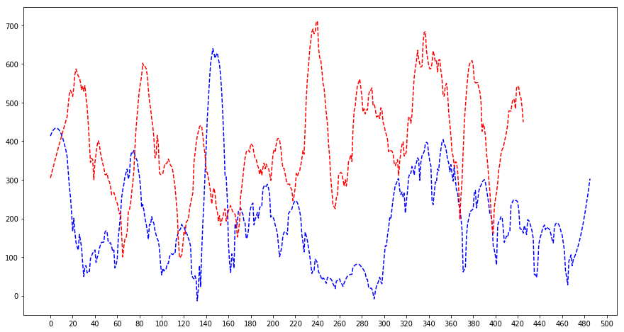
On the first three peaks it can be clearly seen that given that the read dotted line is shifted by ~20 bins the red and blue peaks overlap.
shift = 20

plt.figure(figsize=(15, 8))
plt.plot(np.linspace(shift, 520, len(maximum_dc)), savgol_filter(maximum_dc, 31, 2), 'b--')
plt.plot(savgol_filter(maximum_dc2, 31, 2), 'r--')
plt.xticks(np.linspace(0, 500, 26))
plt.show()
/opt/conda/lib/python3.6/site-packages/scipy/signal/_savitzky_golay.py:187: RankWarning: Polyfit may be poorly conditioned
  xx_edge, polyorder)
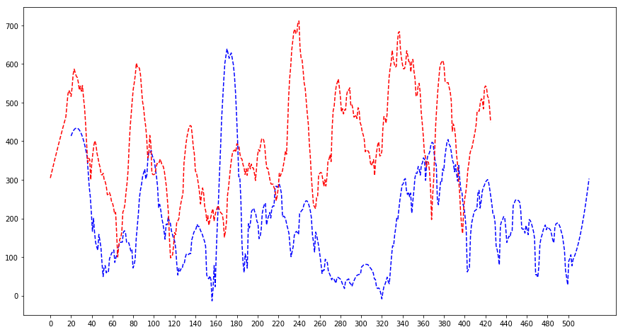
It seems like somewhat working since the first 3 peaks are overlapping as well as the 5th and the 8th and 9th. The last peaks of the dotted blue line are not contained here since some misbehaviour of the smoothing filter. Thus 20 bins means 20 weeks to travel approximately 220 miles for a storm which sounds farfetched so I do not believe my results here. 20 weeks is around a season so I most probably see the changing of seasons here.
@Regards, Alex

Alex Olar
Christian, foodie, physicist, tech enthusiast