
Variational autoencoder on the CIFAR-10 dataset 2.
- 8 minsVariational autoenconder - VAE (2.)
In the previous post I used a vanilla variational autoencoder with little educated guesses and just tried out how to use Tensorflow properly. Since than I got more familiar with it and realized that there are at least 9 versions that are currently supported by the Tensorflow team and the major version 2.0 is released soon.
I was pointed to the direction of building my VAE with the new interface and provided guidence by David Nagy I was successfull with that. I considered using a different reconstruction loss that models colored pictures properly. I used Google Colab to train my model and started an OOP project on move on with my research at Wigner Institute regarding edge generation.
import tensorflow as tf
from tensorflow.keras import layers
import tensorflow_probability as tfp
Tensorflow Probability is a powerful tool that is being developed alongside Tensorflow. It is a probabilistic programming API that is probably going to be the future of deep learning and AI in general.
"""
  Convolutional structure for the encoder net
"""

encoder = tf.keras.Sequential([
    layers.Conv2D(filters=64 , kernel_size=4, strides=2, activation=tf.nn.relu, padding='same'),
    layers.Conv2D(filters=128, kernel_size=4, strides=2, activation=tf.nn.relu, padding='same'),
    layers.Conv2D(filters=512, kernel_size=4, strides=2, activation=tf.nn.relu, padding='same'),
    layers.Flatten()
])

"""
  DeConv structure for the decoder net
"""

decoder = tf.keras.Sequential([
    layers.Dense(2048),
    layers.Reshape(target_shape=(4, 4, 128), input_shape=(None, 1024)),
    layers.Conv2DTranspose(filters=256, kernel_size=4, strides=2, activation=tf.nn.relu, padding='same'),
    layers.Conv2DTranspose(filters=64 , kernel_size=4, strides=2, activation=tf.nn.relu, padding='same'),
    layers.Conv2DTranspose(filters=3  , kernel_size=4, strides=2, activation=tf.nn.relu, padding='same')
])
I used here the Conv2DTranspose layer which is kind of an inverse if the convolutional layers, although they are not injective. It projects the underlying small dimensional dense layer up to the starting resolution of the image. Using this provides much better recontruction that an MLP decoder.
batch_size = 250

x = tf.placeholder(tf.float32, shape=[batch_size, 32, 32, 3])

encoded = encoder(x)

mean = layers.Dense(1024, tf.nn.softplus)(encoded)
sigma = layers.Dense(1024, tf.nn.relu)(encoded)

z = mean + tf.multiply(tf.sqrt(tf.exp(sigma)),
                       tf.random_normal(shape=(batch_size, 1024)))

x_reco = decoder(z)
I am using here the same numerical transformation to acquire a normal prior as before.
reconstruction_term = -tf.reduce_sum(tfp.distributions.MultivariateNormalDiag(
    layers.Flatten()(x_reco), scale_identity_multiplier=0.05).log_prob(layers.Flatten()(x)))

kl_divergence = tf.reduce_sum(tf.keras.metrics.kullback_leibler_divergence(x, x_reco), axis=[1, 2])

cost = tf.reduce_mean(reconstruction_term + kl_divergence)
The API provides a clean interface to compute the KL-divergence and the reconstruction loss. Since I am using colored images and the output is not black-or-white I chose a multivartiate normal distribution provided that the pixels values are independent probabilistic variables only diagonal elements are taken into consideration. The scale_identity_multiplier helpes to keep the variance low and also provides a numeric value to make this VAE more effective, since low varience means more pronounced images.
optimizer = tf.train.AdamOptimizer(learning_rate=0.0001).minimize(cost)
Using AdamOptimizer is almost always the best choice as it implements quite a lot of computational candies to make optimization more efficient.
from tensorflow.keras.datasets.cifar10 import load_data
(X_train, y_train), (X_test, y_test) = load_data()
Downloading data from https://www.cs.toronto.edu/~kriz/cifar-10-python.tar.gz
170500096/170498071 [==============================] - 316s 2us/step
runs = 20
n_minibatches = int(X_train.shape[0] / batch_size)

print("Number of minibatches: ", n_minibatches)

sess = tf.InteractiveSession()
init = tf.global_variables_initializer()
sess.run(init)

for epoch in range(runs):
    pbar = tf.contrib.keras.utils.Progbar(n_minibatches)
    for i in range(n_minibatches):

        x_batch = X_train[i*batch_size:(i+1)*batch_size]/255.
        cost_, _ = sess.run((cost, optimizer), feed_dict={x: x_batch})

        pbar.add(1,[("cost",cost_)])
Number of minibatches:  200


200/200 [==============================] - 27s 133ms/step - cost: 8438750.5125
200/200 [==============================] - 26s 131ms/step - cost: 1886222.4719
200/200 [==============================] - 26s 131ms/step - cost: 1135819.7325
200/200 [==============================] - 26s 131ms/step - cost: 647328.1506
200/200 [==============================] - 26s 131ms/step - cost: 424253.9412
200/200 [==============================] - 26s 131ms/step - cost: 287276.1135
200/200 [==============================] - 26s 131ms/step - cost: 187784.4109
200/200 [==============================] - 26s 130ms/step - cost: 93398.3268
200/200 [==============================] - 26s 130ms/step - cost: 14311.1887
200/200 [==============================] - 26s 131ms/step - cost: -56614.8807
200/200 [==============================] - 26s 130ms/step - cost: -123770.9586
200/200 [==============================] - 26s 130ms/step - cost: -190442.4804
200/200 [==============================] - 26s 130ms/step - cost: -254153.4708
200/200 [==============================] - 26s 130ms/step - cost: -326485.6181
200/200 [==============================] - 26s 129ms/step - cost: -372028.0549
200/200 [==============================] - 26s 129ms/step - cost: -420985.0958
200/200 [==============================] - 26s 130ms/step - cost: -456808.3198
200/200 [==============================] - 26s 130ms/step - cost: -491775.2614
200/200 [==============================] - 26s 130ms/step - cost: -521798.0739
200/200 [==============================] - 26s 130ms/step - cost: -557824.0292
It can be seen that the loss is not yet converged but I only let it run for 20 epochs. Consider this early stopping. :)
import matplotlib.pyplot as plt
import numpy as np

n_rec = 10

x_batch = X_train[0:batch_size]

plt.figure(figsize=(n_rec+6,4))

pred_img = sess.run(x_reco, feed_dict={x: x_batch})
pred_img = pred_img.reshape(batch_size, 32, 32, 3)
pred_img = pred_img.astype(np.int32)

for i in range(n_rec):

    plt.subplot(2, n_rec, i+1)
    plt.imshow(x_batch[i])

    plt.subplot(2, n_rec, n_rec+i+1)
    plt.imshow(pred_img[i])

plt.tight_layout()
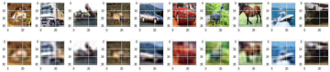
They are somewhat reconstructed, definetely much better than previously with the MLP encoder and decoder. However they are pretty washed out.
@Regards, Alex

Alex Olar
Christian, foodie, physicist, tech enthusiast