
Autoencoders on different datasets - neuroscience
- 34 minsAutoencoders
Autoencoders are used as a new compression tool for images. An ecoder and a decoder network can be trained to learn a lower dimensional representation of the training data set and sevaing the parameters of this lower representation and the decoder network’s weights one can achive much better compression than before.
It is quite hard to find SOTA architectures for AEs so I am only experimenting with very small networks and basic architectures. However, Google has a disentanglement library that is based on variational autoencoders. In the next post I would like to try that properly and build proper variational autoencoders at last.
Methods
The encoder and decoder networks learn a probability distribution from the images to a lower representation vector and a probability distribution from the latent representation back to the reconstructed images. For binarized images the loss should be defined for binary values and such loss is the Bernoulli-distribution. On continuous pixel values a Normal-distribuition can be used as loss function.
Datasets
I am experimenting with texture images from the Wigner CSNL group, the well known MNIST and CIFAR-10 datasets.
from keras.layers import Input, Conv2D, UpSampling2D,\
MaxPooling2D, Dense, Reshape, Flatten, Conv2DTranspose
from keras.models import Model
import tensorflow_probability as tfp
tfd = tfp.distributions
import tensorflow as tf
import keras as K
import pickle
from sklearn.model_selection import train_test_split
import numpy as np
import matplotlib.pyplot as plt
from abc import abstractmethod

with open('../input/textures_42000_28px.pkl', 'rb') as f:
    data = pickle.load(f)

BATCH_SIZE = 128

X_train = data['train_images']
X_test = data['test_images']

# Shuffle
X_train, _ = train_test_split(X_train, test_size=0, random_state=45)
X_test, _ = train_test_split(X_test, test_size=0, random_state=42)
Using TensorFlow backend.
I am defining here a skeleten for all the AutoEncoders that I’m going to use later in this code. Obviously an input_shape and a latent_dim is needed in order to define any AU architecture. The encoder, decoder and model layers should be defined for the particular implementation but the losses are predefined here, such as sigmoid-cross-entropy, bernoulli loss, normal loss and multivariate normal diagonal loss, in the latter two losses the scaling factor is by default learnable as well.
class AutoEncoder:
    def __init__(self, input_shape, latent_dim):
        self.input_shape = input_shape
        self.latent_dim = latent_dim

    @abstractmethod
    def _encoder(self, input_img):
        pass

    @abstractmethod
    def _decoder(self, latent):
        pass

    @abstractmethod
    def get_compiled_model(self, loss_fn=None):
        pass

    def _get_loss(self, loss_fn):
        if loss_fn == None:
            return self._bernoulli
        elif loss_fn == "binary":
            return self._binary
        elif loss_fn == "normal":
            return self._normal
        elif loss_fn == "normalDiag":
            return self._normalDiag

    """
      For binarized input
    """
    def _binary(self, x_true, x_reco):
        return -tf.nn.sigmoid_cross_entropy_with_logits(labels=x_true, logits=x_reco)

    def _bernoulli(self, x_true, x_reco):
        return -tf.reduce_mean(tfd.Bernoulli(x_reco)._log_prob(x_true))

    """
      For non binarized input.
    """
    def _normal(self, x_true, x_reco):
        return -tf.reduce_mean(
            tfd.Normal(x_reco, scale=0.001)._log_prob(x_true))

    def _normalDiag(self, x_true, x_reco):
        return -tf.reduce_mean(
            tfd.MultivariateNormalDiag(x_reco, scale_identity_multiplier=tf.Variable(0.001))._log_prob(x_true))
Here I am defining a Convolutional AE which can be used on (28, 28, 1) images since the architecture is not flexible enough and also, the latent space should be 128 dimensional since I am reshaping it to a (4, 4, 8) matrix.
I’ve read in an article that PReLU performs better than ReLU but I don’t have very high hopes for that.
The decoder’s last layer doesn’t have an activation since the loss functions all expect logits!
################################################################################
class ConvolutionalAutoEncoder(AutoEncoder):
    def _encoder(self, input_img):
        x = Conv2D(512, (2, 2), activation='relu', padding='same')(input_img)
        x = MaxPooling2D((2, 2), padding='same')(x)
        x = Conv2D(256, (2, 2), activation='relu', padding='same')(x)
        x = MaxPooling2D((2, 2), padding='same')(x)
        x = Conv2D(128, (2, 2), activation='relu', padding='same')(x)
        x = MaxPooling2D((2, 2), padding='same')(x)
        encoded = Flatten()(x)
        return encoded

    def _decoder(self, latent):
        x = Reshape((4, 4, 8))(latent)
        x = Conv2DTranspose(128, (2, 2), strides=(2, 2), activation='relu', padding='same')(x)
        x = Conv2D(256, (2, 2), activation='relu')(x)
        x = Conv2DTranspose(512, (2, 2), strides=(2, 2), activation='relu', padding='same')(x)
        reco = Conv2DTranspose(1, (2, 2), strides=(2, 2))(x)
        return reco

    def get_compiled_model(self, loss_fn=None):
        self.loss_fn = super()._get_loss(loss_fn)
        input_img = Input(shape=self.input_shape)
        encoded = self._encoder(input_img)
        latent = Dense(self.latent_dim)(encoded)
        reco = self._decoder(latent)
        model = Model(input_img, reco)
        model.compile(optimizer='adadelta', loss=self.loss_fn)
        return model
################################################################################
For the CIFAR-10 dataset I needed another implementation since the different input_shape, which is a 3-channeled image and the different architecture. This part should be generalized in the future.
################################################################################
class ConvolutionalAutoEncoderCIFAR(AutoEncoder):

    def _encoder(self, input_img):
        x = Conv2D(512, (2, 2), activation='relu', padding='same')(input_img)
        x = MaxPooling2D((2, 2), padding='same')(x)
        x = Conv2D(256, (2, 2), activation='relu', padding='same')(x)
        x = MaxPooling2D((2, 2), padding='same')(x)
        x = Conv2D(128, (2, 2), activation='relu', padding='same')(x)
        x = MaxPooling2D((2, 2), padding='same')(x)
        encoded = Flatten()(x)
        return encoded

    def _decoder(self, latent):
        x = Reshape((4, 4, 16))(latent)
        x = Conv2DTranspose(256, (2, 2), strides=(2, 2), activation='relu', padding='same')(x)
        x = Conv2DTranspose(512, (2, 2), strides=(2, 2), activation='relu', padding='same')(x)
        x = Conv2DTranspose(1024, (2, 2), strides=(2, 2), activation='relu', padding='same')(x)
        reco = Conv2D(3, (2, 2), padding='same')(x)
        return reco

    def get_compiled_model(self, loss_fn=None):
        self.loss_fn = super()._get_loss(loss_fn)
        input_img = Input(shape=self.input_shape)
        encoded = self._encoder(input_img)
        latent = Dense(self.latent_dim)(encoded)
        reco = self._decoder(latent)
        model = Model(input_img, reco)
        model.compile(optimizer='adadelta', loss=self.loss_fn)
        return model
################################################################################
Also I am experimenting with a dense AE which is more flexible than the previous two and basically any type of flattened input can be fed to it.
################################################################################
class DenseAutoEncoder(AutoEncoder):

    def _encoder(self, input_tensor):
        x = Dense(512, activation='relu')(input_tensor)
        x = Dense(256, activation='relu')(x)
        return x

    def _decoder(self, latent):
        x = Dense(256, activation='relu')(latent)
        x = Dense(512, activation='relu')(x)
        reco = Dense(self.input_shape[1])(x)
        return reco

    def get_compiled_model(self, loss_fn=None):
        self.loss_fn = super()._get_loss(loss_fn)
        input_tensor = Input(shape=(self.input_shape[1],))
        encoded = self._encoder(input_tensor)
        latent = Dense(self.latent_dim)(encoded)
        reco = self._decoder(latent)
        model = Model(input_tensor, reco)
        model.compile(optimizer='adam', loss=self.loss_fn)
        return model
################################################################################
An image preprocessing class that can feed batches in proper format for the different models.
from keras.preprocessing.image import ImageDataGenerator

class DataGenerator:
    def __init__(self, train, test, BATCH_SIZE=128, IMAGE_SHAPE=(28, 28, 1)):
        self.DATAGEN = ImageDataGenerator()
        self.IMAGE_SHAPE = IMAGE_SHAPE
        self.BATCH_SIZE = BATCH_SIZE

        self.train = train
        self.test = test

        self._train = train.reshape(X_train.shape[0], *IMAGE_SHAPE)
        self._test = test.reshape(X_test.shape[0], *IMAGE_SHAPE)

    def flow(self):
        return self.DATAGEN.flow(self._train, self._train, batch_size=self.BATCH_SIZE)

    def flatten_flow(self):
        def train_generator(_it):
            image_dim = self.IMAGE_SHAPE[0]*self.IMAGE_SHAPE[1]*self.IMAGE_SHAPE[2]
            while True:
                batch_x, batch_y = next(_it)
                yield batch_x.reshape(batch_x.shape[0], image_dim), batch_y.reshape(batch_y.shape[0], image_dim)
        return train_generator(self.flow())

    def validation_data(self):
        return self._test, self._test

    def flattened_validation_data(self):
        return self.test, self.test
1. Textures - Wigner CSNL
textures = DataGenerator(X_train, X_test)

flow = textures.flow()
flatten_flow = textures.flatten_flow()

validation_data = textures.validation_data()
flattened_validation_data = textures.flattened_validation_data()
Since the images have continous pixel values I’ll use a Normal-distribution for the loss.
autoencoder = ConvolutionalAutoEncoder(input_shape=(28, 28, 1), latent_dim=4*4*8)
model = autoencoder.get_compiled_model("normal")
model.summary()
_________________________________________________________________
Layer (type)                 Output Shape              Param #
=================================================================
input_1 (InputLayer)         (None, 28, 28, 1)         0
_________________________________________________________________
conv2d_1 (Conv2D)            (None, 28, 28, 512)       2560
_________________________________________________________________
max_pooling2d_1 (MaxPooling2 (None, 14, 14, 512)       0
_________________________________________________________________
conv2d_2 (Conv2D)            (None, 14, 14, 256)       524544
_________________________________________________________________
max_pooling2d_2 (MaxPooling2 (None, 7, 7, 256)         0
_________________________________________________________________
conv2d_3 (Conv2D)            (None, 7, 7, 128)         131200
_________________________________________________________________
max_pooling2d_3 (MaxPooling2 (None, 4, 4, 128)         0
_________________________________________________________________
flatten_1 (Flatten)          (None, 2048)              0
_________________________________________________________________
dense_1 (Dense)              (None, 128)               262272
_________________________________________________________________
reshape_1 (Reshape)          (None, 4, 4, 8)           0
_________________________________________________________________
conv2d_transpose_1 (Conv2DTr (None, 8, 8, 128)         4224
_________________________________________________________________
conv2d_4 (Conv2D)            (None, 7, 7, 256)         131328
_________________________________________________________________
conv2d_transpose_2 (Conv2DTr (None, 14, 14, 512)       524800
_________________________________________________________________
conv2d_transpose_3 (Conv2DTr (None, 28, 28, 1)         2049
=================================================================
Total params: 1,582,977
Trainable params: 1,582,977
Non-trainable params: 0
_________________________________________________________________
And fitting it…
history = model.fit_generator(
    flow,
    steps_per_epoch=250, verbose=1, epochs=120, validation_data=validation_data)
Epoch 1/120
250/250 [==============================] - 11s 45ms/step - loss: 23619.4608 - val_loss: 13064.3834
Epoch 2/120
250/250 [==============================] - 9s 34ms/step - loss: 12936.3868 - val_loss: 12984.5468

######################################################################################
##############  THESE LINES WERE INTENTIONALLY LEFT OUT ##############################
######################################################################################

Epoch 45/120
250/250 [==============================] - 8s 34ms/step - loss: 8065.7741 - val_loss: 8895.6037
Epoch 46/120
250/250 [==============================] - 8s 34ms/step - loss: 8037.6332 - val_loss: 8693.5458
Epoch 47/120
250/250 [==============================] - 8s 34ms/step - loss: 7969.5045 - val_loss: 8657.9726
Epoch 48/120
142/250 [================>.............] - ETA: 3s - loss: 8082.0893
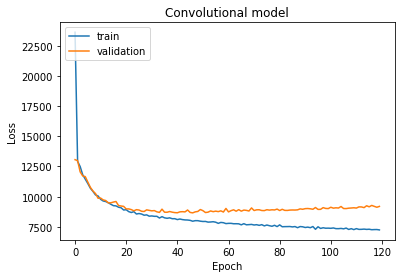
It can be seen that around 30 epochs the validation loss is minimal after that the algorithm overfits.
# "Accuracy"
plt.title("Convolutional model")
plt.plot(history.history['loss'])
plt.plot(history.history['val_loss'])
plt.ylabel('Loss')
plt.xlabel('Epoch')
plt.legend(['train', 'validation'], loc='upper left')
plt.show()
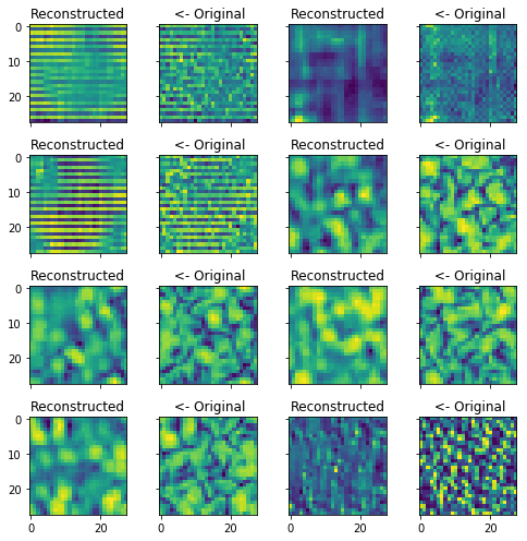
Reconstucting the training set shows that the algorithm works the reconstructed images are very vague.
reco = model.predict(X_train[:BATCH_SIZE].reshape(BATCH_SIZE, 28, 28, 1))

fig, axes = plt.subplots(4, 4, sharex=True, sharey=True, figsize=(7, 7))

for ind, ax in enumerate(axes.flatten()):
  if ind % 2 == 0:
    ax.set_title('Reconstructed')
    ax.imshow(reco[ind].reshape(28, 28))
  else:
    ax.set_title(' <- Original')
    ax.imshow(X_train[ind - 1].reshape(28, 28))
fig.tight_layout()
plt.show()
Using the dense model:
autoencoder = DenseAutoEncoder(input_shape=(None, 28*28*1), latent_dim=128)
model = autoencoder.get_compiled_model("normal")
model.summary()
_________________________________________________________________
Layer (type)                 Output Shape              Param #
=================================================================
input_2 (InputLayer)         (None, 784)               0
_________________________________________________________________
dense_2 (Dense)              (None, 512)               401920
_________________________________________________________________
dense_3 (Dense)              (None, 256)               131328
_________________________________________________________________
dense_4 (Dense)              (None, 128)               32896
_________________________________________________________________
dense_5 (Dense)              (None, 256)               33024
_________________________________________________________________
dense_6 (Dense)              (None, 512)               131584
_________________________________________________________________
dense_7 (Dense)              (None, 784)               402192
=================================================================
Total params: 1,132,944
Trainable params: 1,132,944
Non-trainable params: 0
_________________________________________________________________
history = model.fit_generator(
    flatten_flow,
    steps_per_epoch=450, verbose=1, epochs=120, validation_data=flattened_validation_data)
Epoch 1/120
450/450 [==============================] - 3s 6ms/step - loss: 13660.7373 - val_loss: 12234.5759
Epoch 2/120
450/450 [==============================] - 2s 5ms/step - loss: 11909.9524 - val_loss: 11495.2333
Epoch 3/120
450/450 [==============================] - 2s 5ms/step - loss: 11203.8561 - val_loss: 11164.1901

######################################################################################
##############  THESE LINES WERE INTENTIONALLY LEFT OUT ##############################
######################################################################################

Epoch 118/120
450/450 [==============================] - 2s 5ms/step - loss: 8678.0076 - val_loss: 9734.9756
Epoch 119/120
450/450 [==============================] - 2s 5ms/step - loss: 8731.5442 - val_loss: 9700.1280
Epoch 120/120
450/450 [==============================] - 2s 5ms/step - loss: 8662.2679 - val_loss: 9717.2447
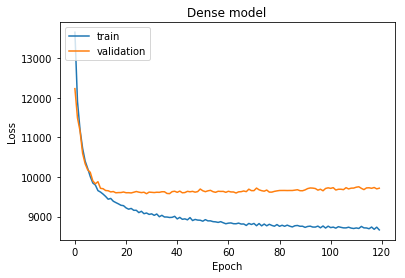
# "Accuracy"
plt.title("Dense model")
plt.plot(history.history['loss'])
plt.plot(history.history['val_loss'])
plt.ylabel('Loss')
plt.xlabel('Epoch')
plt.legend(['train', 'validation'], loc='upper left')
plt.show()
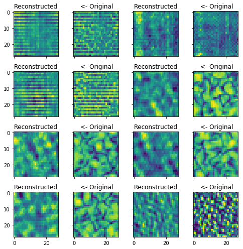
reco = model.predict(X_train[:BATCH_SIZE])

fig, axes = plt.subplots(4, 4, sharex=True, sharey=True, figsize=(7, 7))

for ind, ax in enumerate(axes.flatten()):
  if ind % 2 == 0:
    ax.set_title('Reconstructed')
    ax.imshow(reco[ind].reshape(28, 28))
  else:
    ax.set_title(' <- Original')
    ax.imshow(X_train[ind - 1].reshape(28, 28))
fig.tight_layout()
plt.show()
General structure, shades and shapes are somewhat reconstructed but overall very poor performance. Actually I have no idea whether or not I should see this or I am just messing up something.
To find out whether or not I am doing huge BS I am moving on to the MNIST dataset on which the models should perform far better and almost should give me back pixel perfect representations due to the simplicity of the images.
###########################################################################
########################         MNIST          ###########################
###########################################################################

from keras.datasets.mnist import load_data

(X_train, _), (X_test, _) = load_data()

X_train = X_train.reshape(X_train.shape[0], 784)
X_test = X_test.reshape(X_test.shape[0], 784)

X_train = X_train / 255.
X_test = X_test / 255.
Downloading data from https://s3.amazonaws.com/img-datasets/mnist.npz
11493376/11490434 [==============================] - 1s 0us/step
After the acquiry of the data I am going to train a dense model with normal loss since the pixel values are continous. In the Tensorflow guide and almost everywhere on the web when people trained these models they binarized the MNIST input and used binary losses such as the Bernoulli-loss. With that a much better representation can be learned and the reconstruction is also far superior.
mnist = DataGenerator(X_train, X_test)
autoencoder = DenseAutoEncoder(input_shape=(None, 28*28), latent_dim=16)
model = autoencoder.get_compiled_model("normal")
model.summary()
_________________________________________________________________
Layer (type)                 Output Shape              Param #
=================================================================
input_3 (InputLayer)         (None, 784)               0
_________________________________________________________________
dense_8 (Dense)              (None, 512)               401920
_________________________________________________________________
dense_9 (Dense)              (None, 256)               131328
_________________________________________________________________
dense_10 (Dense)             (None, 16)                4112
_________________________________________________________________
dense_11 (Dense)             (None, 256)               4352
_________________________________________________________________
dense_12 (Dense)             (None, 512)               131584
_________________________________________________________________
dense_13 (Dense)             (None, 784)               402192
=================================================================
Total params: 1,075,488
Trainable params: 1,075,488
Non-trainable params: 0
_________________________________________________________________
history = model.fit_generator(
    mnist.flatten_flow(),
    steps_per_epoch=350, verbose=1, epochs=150, validation_data=mnist.flattened_validation_data())
Epoch 1/150
350/350 [==============================] - 2s 7ms/step - loss: 15142.9858 - val_loss: 10154.8432
Epoch 2/150
350/350 [==============================] - 2s 5ms/step - loss: 9418.3889 - val_loss: 8631.6228

######################################################################################
##############  THESE LINES WERE INTENTIONALLY LEFT OUT ##############################
######################################################################################

Epoch 149/150
350/350 [==============================] - 2s 5ms/step - loss: 3862.4324 - val_loss: 4313.8704
Epoch 150/150
350/350 [==============================] - 2s 6ms/step - loss: 3883.1469 - val_loss: 4325.9544
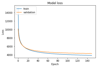
print(history.history.keys())

# "Accuracy"
plt.plot(history.history['loss'])
plt.plot(history.history['val_loss'])
plt.title('Model loss')
plt.ylabel('Loss')
plt.xlabel('Epoch')
plt.legend(['train', 'validation'], loc='upper left')
plt.show()
dict_keys(['val_loss', 'loss'])
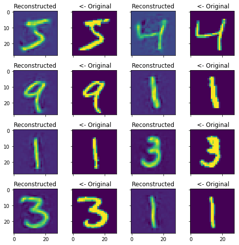
reco = model.predict(X_train[:BATCH_SIZE].reshape(BATCH_SIZE, 28*28))
fig, axes = plt.subplots(4, 4, sharex=True, sharey=True, figsize=(7, 7))

for ind, ax in enumerate(axes.flatten()):
  if ind % 2 == 0:
    ax.set_title('Reconstructed')
    ax.imshow(reco[ind].reshape(28, 28))
  else:
    ax.set_title(' <- Original')
    ax.imshow(X_train[ind - 1].reshape(28, 28))
fig.tight_layout()
plt.show()
The training reconstruction looks quite OK since with supression filter the somewhat brights spots can be eliminated and the reconstructed digits would look almost exactly the same.
Moving on to a convolutional architecture:
autoencoder2 = ConvolutionalAutoEncoder(input_shape=(28, 28, 1), latent_dim=128)
model2 = autoencoder2.get_compiled_model("normal")
model2.summary()
<bound method AutoEncoder._normal of <__main__.ConvolutionalAutoEncoder object at 0x7f70787187f0>>
_________________________________________________________________
Layer (type)                 Output Shape              Param #
=================================================================
input_4 (InputLayer)         (None, 28, 28, 1)         0
_________________________________________________________________
conv2d_5 (Conv2D)            (None, 28, 28, 512)       2560
_________________________________________________________________
max_pooling2d_4 (MaxPooling2 (None, 14, 14, 512)       0
_________________________________________________________________
conv2d_6 (Conv2D)            (None, 14, 14, 256)       524544
_________________________________________________________________
max_pooling2d_5 (MaxPooling2 (None, 7, 7, 256)         0
_________________________________________________________________
conv2d_7 (Conv2D)            (None, 7, 7, 128)         131200
_________________________________________________________________
max_pooling2d_6 (MaxPooling2 (None, 4, 4, 128)         0
_________________________________________________________________
flatten_2 (Flatten)          (None, 2048)              0
_________________________________________________________________
dense_14 (Dense)             (None, 128)               262272
_________________________________________________________________
reshape_2 (Reshape)          (None, 4, 4, 8)           0
_________________________________________________________________
conv2d_transpose_4 (Conv2DTr (None, 8, 8, 128)         4224
_________________________________________________________________
conv2d_8 (Conv2D)            (None, 7, 7, 256)         131328
_________________________________________________________________
conv2d_transpose_5 (Conv2DTr (None, 14, 14, 512)       524800
_________________________________________________________________
conv2d_transpose_6 (Conv2DTr (None, 28, 28, 1)         2049
=================================================================
Total params: 1,582,977
Trainable params: 1,582,977
Non-trainable params: 0
_________________________________________________________________
history = model2.fit_generator(
    mnist.flow(),
    steps_per_epoch=300, verbose=1,
    epochs=100, validation_data=mnist.validation_data())
Epoch 1/100
300/300 [==============================] - 12s 39ms/step - loss: 26276.0108 - val_loss: 15903.1574
Epoch 2/100
300/300 [==============================] - 11s 36ms/step - loss: 10832.0214 - val_loss: 7923.0541

######################################################################################
##############  THESE LINES WERE INTENTIONALLY LEFT OUT ##############################
######################################################################################

Epoch 81/100
300/300 [==============================] - 11s 35ms/step - loss: 1382.4032 - val_loss: 1738.3417
Epoch 82/100
229/300 [=====================>........] - ETA: 2s - loss: 1380.0090
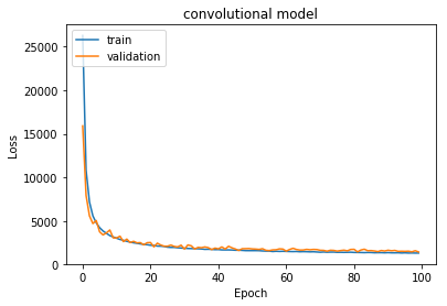
plt.title("convolutional model")
plt.plot(history.history['loss'])
plt.plot(history.history['val_loss'])
plt.ylabel('Loss')
plt.xlabel('Epoch')
plt.legend(['train', 'validation'], loc='upper left')
plt.show()
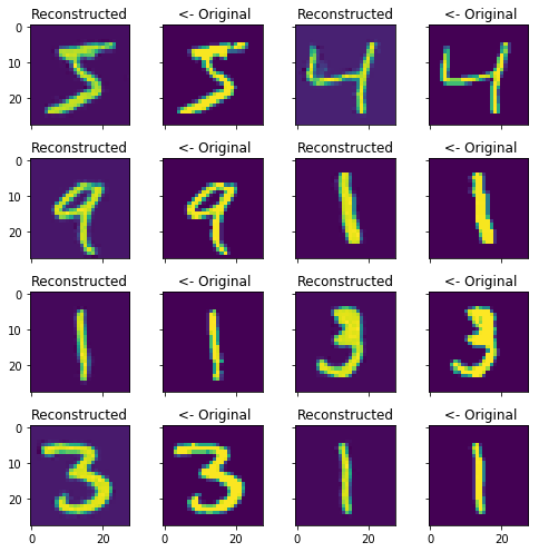
"""
    Train set reconstruction.
"""

reco = model2.predict(X_train[:BATCH_SIZE].reshape(BATCH_SIZE, 28, 28, 1))

fig, axes = plt.subplots(4, 4, sharex=True, sharey=True, figsize=(7, 7))

for ind, ax in enumerate(axes.flatten()):
  if ind % 2 == 0:
    ax.set_title('Reconstructed')
    ax.imshow(reco[ind].reshape(28, 28))
  else:
    ax.set_title(' <- Original')
    ax.imshow(X_train[ind - 1].reshape(28, 28))
fig.tight_layout()
plt.show()
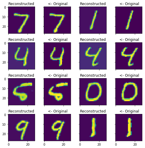
The reconstruction is almost pixel perfect without supression on bright spots and also very good on the test set which was previously unseen and not learned by the system.
"""
    Test set reconstruction.
"""

reco = model2.predict(X_test[:BATCH_SIZE].reshape(BATCH_SIZE, 28, 28, 1))

fig, axes = plt.subplots(4, 4, sharex=True, sharey=True, figsize=(7, 7))

for ind, ax in enumerate(axes.flatten()):
  if ind % 2 == 0:
    ax.set_title('Reconstructed')
    ax.imshow(reco[ind].reshape(28, 28))
  else:
    ax.set_title(' <- Original')
    ax.imshow(X_test[ind - 1].reshape(28, 28))
fig.tight_layout()
plt.show()
However, almost everything performs well on MNIST so I am not convinced that I am not messing up something with my models. In order to find out I am moving on to the CIFAR-10 dataset which consists of 10 different types of image classes and also RGB so I assume that it is much more abstract then MNIST or Wigner CSNL Textures. I’m expecting that the reconstruction should therefore by worse or on par with texture reconstructions.
##########################
"""
    Trying with cifar-10
"""
##########################

from keras.datasets.cifar10 import load_data
(X_train, _), (X_test, _) = load_data()

X_train = X_train.reshape(X_train.shape[0], 32*32*3)
X_test = X_test.reshape(X_test.shape[0], 32*32*3)

X_train = X_train / 255.
X_test = X_test / 255.
Downloading data from https://www.cs.toronto.edu/~kriz/cifar-10-python.tar.gz
170500096/170498071 [==============================] - 66s 0us/step
cifar = DataGenerator(X_train, X_test, BATCH_SIZE=128, IMAGE_SHAPE=(32, 32, 3))
Only trying the convolutional model since the dense model would take more time and is less flexible. Also using 256 as latent dimension size, since the input images are 32323 dimensional which is much higher than the previously used 28*28 input dimensions.
autoencoder3 = ConvolutionalAutoEncoderCIFAR(input_shape=(32, 32, 3), latent_dim=256)
model3 = autoencoder3.get_compiled_model("normal")
model3.summary()
_________________________________________________________________
Layer (type)                 Output Shape              Param #
=================================================================
input_5 (InputLayer)         (None, 32, 32, 3)         0
_________________________________________________________________
conv2d_9 (Conv2D)            (None, 32, 32, 512)       6656
_________________________________________________________________
max_pooling2d_7 (MaxPooling2 (None, 16, 16, 512)       0
_________________________________________________________________
conv2d_10 (Conv2D)           (None, 16, 16, 256)       524544
_________________________________________________________________
max_pooling2d_8 (MaxPooling2 (None, 8, 8, 256)         0
_________________________________________________________________
conv2d_11 (Conv2D)           (None, 8, 8, 128)         131200
_________________________________________________________________
max_pooling2d_9 (MaxPooling2 (None, 4, 4, 128)         0
_________________________________________________________________
flatten_3 (Flatten)          (None, 2048)              0
_________________________________________________________________
dense_15 (Dense)             (None, 256)               524544
_________________________________________________________________
reshape_3 (Reshape)          (None, 4, 4, 16)          0
_________________________________________________________________
conv2d_transpose_7 (Conv2DTr (None, 8, 8, 256)         16640
_________________________________________________________________
conv2d_transpose_8 (Conv2DTr (None, 16, 16, 512)       524800
_________________________________________________________________
conv2d_transpose_9 (Conv2DTr (None, 32, 32, 1024)      2098176
_________________________________________________________________
conv2d_12 (Conv2D)           (None, 32, 32, 3)         12291
=================================================================
Total params: 3,838,851
Trainable params: 3,838,851
Non-trainable params: 0
_________________________________________________________________
history = model3.fit_generator(
    cifar.flow(),
    steps_per_epoch=450, verbose=1,
    epochs=60, validation_data=cifar.validation_data())
This takes quite a while to train for several epochs but a lot of free cloud GPU compute power is available on Kaggle so I can do this at home.
Epoch 1/60
450/450 [==============================] - 68s 151ms/step - loss: 27946.8238 - val_loss: 14479.2754

######################################################################################
##############  THESE LINES WERE INTENTIONALLY LEFT OUT ##############################
######################################################################################

Epoch 27/60
450/450 [==============================] - 66s 146ms/step - loss: 3538.4969 - val_loss: 3507.9565
Epoch 28/60
284/450 [=================>............] - ETA: 22s - loss: 3480.6532
plt.plot(history.history['loss'])
plt.plot(history.history['val_loss'])
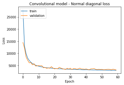
plt.title('Convolutional model - Normal diagonal loss')
plt.ylabel('Loss')
plt.xlabel('Epoch')
plt.legend(['train', 'validation'], loc='upper left')
plt.show()
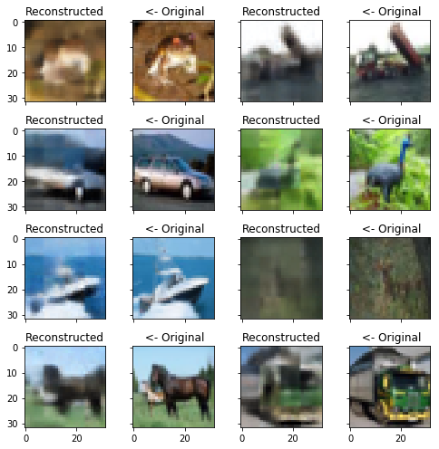
"""
    Train set reconstruction.
"""

reco = model3.predict(X_train[:BATCH_SIZE].reshape(BATCH_SIZE, 32, 32, 3))

fig, axes = plt.subplots(4, 4, sharex=True, sharey=True, figsize=(7, 7))

for ind, ax in enumerate(axes.flatten()):
  if ind % 2 == 0:
    ax.set_title('Reconstructed')
    ax.imshow(reco[ind].reshape(32, 32, 3))
  else:
    ax.set_title(' <- Original')
    ax.imshow(X_train[ind - 1].reshape(32, 32, 3))
fig.tight_layout()
plt.show()
Clipping input data to the valid range for imshow with RGB data ([0..1] for floats or [0..255] for integers).
Clipping input data to the valid range for imshow with RGB data ([0..1] for floats or [0..255] for integers).
Clipping input data to the valid range for imshow with RGB data ([0..1] for floats or [0..255] for integers).
Clipping input data to the valid range for imshow with RGB data ([0..1] for floats or [0..255] for integers).
Clipping input data to the valid range for imshow with RGB data ([0..1] for floats or [0..255] for integers).
Train reconstruction seems to be pretty good especially on the ship and the truch but the deer is not properly captured also the train is very dim.
"""
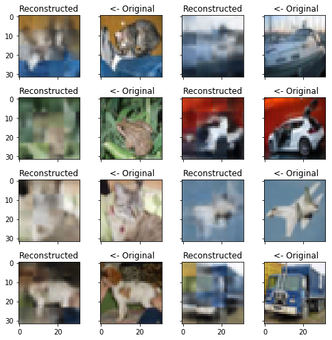
Test set reconstruction.
"""
reco = model3.predict(X_test[:BATCH_SIZE].reshape(BATCH_SIZE, 32, 32, 3))
fig, axes = plt.subplots(4, 4, sharex=True, sharey=True, figsize=(7, 7))
for ind, ax in enumerate(axes.flatten()):
if ind % 2 == 0:
ax.set_title('Reconstructed')
ax.imshow(reco[ind].reshape(32, 32, 3))
else:
ax.set_title(' <- Original')
ax.imshow(X_test[ind - 1].reshape(32, 32, 3))
fig.tight_layout()
plt.show()
Clipping input data to the valid range for imshow with RGB data ([0..1] for floats or [0..255] for integers).
Clipping input data to the valid range for imshow with RGB data ([0..1] for floats or [0..255] for integers).
However the models seems to generalize well, since the truch and the car and also the military plane can be ‘guessed’ from the reconstructed images.
I’ll be moving on with modifying my autoencoders and making them variational and also I’ll be looking for better architextures on arxiv-sanity check from Andrej Karpathy to find great articles on the topic.
@Regards, Alex

Alex Olar
Christian, foodie, physicist, tech enthusiast