
Stacked boosting for photo-z estimation - a university Kaggle challenge
- 14 minsStacked boosting for photo-z estimation - Kaggle challenge
On Kaggle there are many challenges to choose from and it is very easy to host an InClass one. That’s what my teachers (now collegues) did. Recently I was absorbed by university duties and did a fair amount of work, collaboration and study. I couldn’t write a post for a month. :’(
The problem here is very familiar since I’ve worked with this before and I was suprised by how much it can be improved. Ensembling is the way to go. Here is my solution to the challenge and also here’s the link to it.
The best solution was using several stacked MLPs but as teachers said stacked random forests were the way to go. My solution is presented below and was ran on Kaggle.
!nvidia-smi
Sat Mar 30 09:12:08 2019
+-----------------------------------------------------------------------------+
| NVIDIA-SMI 410.104      Driver Version: 410.104      CUDA Version: 10.0     |
|-------------------------------+----------------------+----------------------+
| GPU  Name        Persistence-M| Bus-Id        Disp.A | Volatile Uncorr. ECC |
| Fan  Temp  Perf  Pwr:Usage/Cap|         Memory-Usage | GPU-Util  Compute M. |
|===============================+======================+======================|
|   0  Tesla P100-PCIE...  On   | 00000000:00:04.0 Off |                    0 |
| N/A   49C    P0    30W / 250W |      0MiB / 16280MiB |      0%      Default |
+-------------------------------+----------------------+----------------------+

+-----------------------------------------------------------------------------+
| Processes:                                                       GPU Memory |
|  GPU       PID   Type   Process name                             Usage      |
|=============================================================================|
|  No running processes found                                                 |
+-----------------------------------------------------------------------------+
import numpy as np
import pandas as pd

import os
print(os.listdir("../input"))
['test.csv', 'train.csv', 'sample.csv']
Importing all the necesary sklearn functions and classes. The dataframe is presented below, I also created ug, gr, ri, iz colors since that’s a common way of describing this spectra (feature engineering).
from xgboost import XGBRegressor
from sklearn.model_selection import RandomizedSearchCV
from sklearn.model_selection import train_test_split
from sklearn.preprocessing import normalize, RobustScaler, StandardScaler
from sklearn.pipeline import make_pipeline
from sklearn.ensemble import GradientBoostingRegressor
from sklearn.ensemble import RandomForestRegressor
from catboost import CatBoostRegressor
from sklearn.ensemble import AdaBoostRegressor
import lightgbm as lgb
import pandas as pd
from scipy.stats import uniform, randint

df = pd.read_csv('../input/train.csv')
df.head(n=10)
| ra | dec | u | g | r | i | z | size | ellipticity | redshift | id | |
|---|---|---|---|---|---|---|---|---|---|---|---|
| 0 | 216.0587 | 62.2653 | 19.97 | 18.76 | 17.78 | 17.30 | 16.95 | 11.25 | 0.23 | 0.183 | 0 |
| 1 | 43.9829 | 20.4813 | 19.85 | 17.92 | 16.69 | 16.21 | 15.84 | 9.08 | 0.15 | 0.178 | 1 |
| 2 | 355.8473 | 359.0946 | 19.61 | 18.99 | 18.20 | 17.76 | 17.46 | 2.04 | 0.13 | 0.342 | 2 |
| 3 | 223.1833 | 36.0321 | 22.92 | 20.45 | 18.90 | 18.23 | 17.88 | 7.47 | 0.43 | 0.400 | 3 |
| 4 | 41.6911 | 39.4769 | 22.17 | 22.07 | 20.47 | 19.30 | 18.99 | 12.54 | 0.59 | 0.605 | 4 |
| 5 | 193.0652 | 32.2492 | 19.58 | 18.39 | 17.73 | 17.35 | 17.13 | 4.27 | 0.15 | 0.115 | 5 |
| 6 | 51.6667 | 13.4588 | 20.34 | 18.71 | 17.44 | 16.95 | 16.61 | 11.22 | 0.49 | 0.271 | 6 |
| 7 | 52.0553 | 16.0821 | 23.38 | 20.67 | 19.04 | 18.40 | 18.08 | 2.31 | 0.06 | 0.319 | 7 |
| 8 | 88.5624 | 356.0842 | 19.20 | 17.14 | 16.13 | 15.70 | 15.36 | 8.14 | 0.05 | 0.121 | 8 |
| 9 | 183.3186 | 49.9559 | 22.94 | 21.78 | 20.49 | 19.57 | 19.20 | 7.27 | 0.15 | 0.543 | 9 |
df['ug'] = df['u'] - df['g']
df['gr'] = df['g'] - df['r']
df['ri'] = df['r'] - df['i']
df['iz'] = df['i'] - df['z']

relevant_variables = ['ug', 'gr', 'ri', 'iz', 'ellipticity', 'size', 'r']
I choose those afterwards to be relevant_variables since they encode all the color filters.
The main function is a stack of different boosted moodels on different random samples of the dataset in each iteration.
def bagged_models(N = 1):

    models = []
    rmses = []

    for i in range(N):

        X = df.sample(350_000, random_state=137*N + 4134)

        X_train, X_test, y_train, y_test = train_test_split(
            X[relevant_variables],
            X['redshift'],
            test_size=0.5,
            random_state=42*N)

        # XGB models
        xgb_model = XGBRegressor(tree_method = "gpu_exact", max_depth=11,
                                 reg_lambda=0.9, reg_alpha=0.3, n_estimators=80)

        #xgb_model = make_pipeline(RobustScaler(), xgb_model)

        xgb_model.fit(X_train, y_train)

        pred = xgb_model.predict(X_test)
        mse = mean_squared_error(pred, y_test)

        rmses.append(np.sqrt(mse))
        models.append(xgb_model)

        # LightGBM
        lgbm = lgb.LGBMRegressor(n_estimators=80, max_depth=15,
                                num_leaves=19, reg_alpha=0.4,
                                subsample=0.65, reg_lambda=0.5, silent=True)

        #lgbm = make_pipeline(RobustScaler(), lgbm)

        lgbm.fit(X_train, y_train)

        pred = lgbm.predict(X_test)
        mse = mean_squared_error(pred, y_test)

        rmses.append(np.sqrt(mse))
        models.append(lgbm)

        # GradBoost models
        gb = GradientBoostingRegressor(n_estimators=137, subsample=0.25,
                                       validation_fraction=0.5, max_depth=7,
                                       min_samples_leaf=3)

        #gb = make_pipeline(RobustScaler(), gb)

        gb.fit(X_train, y_train)

        pred = gb.predict(X_test)
        mse = mean_squared_error(pred, y_test)

        rmses.append(np.sqrt(mse))
        models.append(gb)

        # CatBoost models
        cb = CatBoostRegressor(depth=15, early_stopping_rounds=3,
                               loss_function='RMSE', learning_rate=0.1,
                               task_type = "GPU", n_estimators=80, silent=True)

        #cb = make_pipeline(RobustScaler(), gb)

        cb.fit(X_train, y_train)

        pred = cb.predict(X_test)
        mse = mean_squared_error(pred, y_test)

        rmses.append(np.sqrt(mse))
        models.append(cb)

    return models, rmses
import warnings
from sklearn.metrics import mean_squared_error
warnings.filterwarnings('ignore')
models, rmses = bagged_models(N=75)
X_train, X_test, y_train, y_test = train_test_split(
            df[relevant_variables],
            df['redshift'],
            test_size=0.33,
            random_state=42)
Prediction is done for all the models (75 * #number_of_different_types_of_models) on the whole test set..
preds_ = np.array([models[i].predict(X_test) for i in range(0, len(models), 1)])
preds = np.mean(preds_, axis=0)
Arbitrary check to see whether or not stacking worked at all.
np.sqrt(mean_squared_error(preds, y_test)), np.mean(rmses), np.min(rmses), np.argmin(rmses)
(0.045304009089382945, 0.04656930089201668, 0.04613510069939869, 0)
import matplotlib.pyplot as plt
plt.figure(figsize=(12, 9))
plt.hist(y_test, bins=100, color='b')
plt.hist(preds, bins=100, color='r', alpha=0.55)
plt.show()
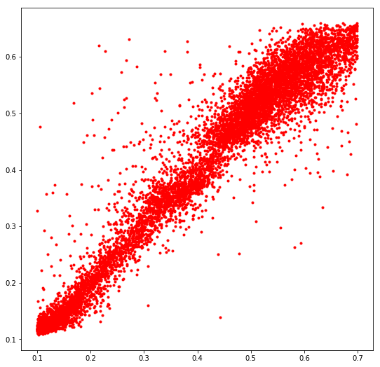
plt.figure(figsize=(9, 9))
plt.plot(y_test[::40], preds[::40], 'r.')
plt.show()
It can be seen that the model does not fit the actual distribution very well and is error prone for outliers. The right tail is completely missed.
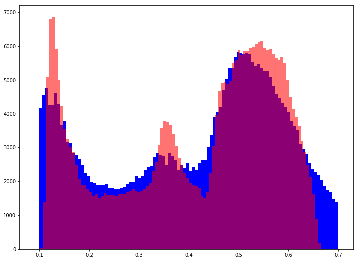
Not all data points are shown since there are very many and the plot looks terrible if all are present.
test_df = pd.read_csv('../input/test.csv')

test_df['ug'] = test_df['u'] - test_df['g']
test_df['gr'] = test_df['g'] - test_df['r']
test_df['ri'] = test_df['r'] - test_df['i']
test_df['iz'] = test_df['i'] - test_df['z']

test_data = test_df[relevant_variables]
Running the prediction on the actual test set then getting the mean of all model predictions.
test_preds = [model.predict(test_data) for model in models]
test_preds = np.mean(test_preds, axis=0)
test_pred = pd.DataFrame(test_preds, columns=['redshift'])
test_pred.to_csv('predictions.csv', index_label='id', columns=['redshift'])
pd.read_csv('predictions.csv').head(n=10)
| id | redshift | |
|---|---|---|
| 0 | 0 | 0.589428 |
| 1 | 1 | 0.252857 |
| 2 | 2 | 0.603094 |
| 3 | 3 | 0.623349 |
| 4 | 4 | 0.141112 |
| 5 | 5 | 0.527417 |
| 6 | 6 | 0.436981 |
| 7 | 7 | 0.343215 |
| 8 | 8 | 0.342766 |
| 9 | 9 | 0.539182 |
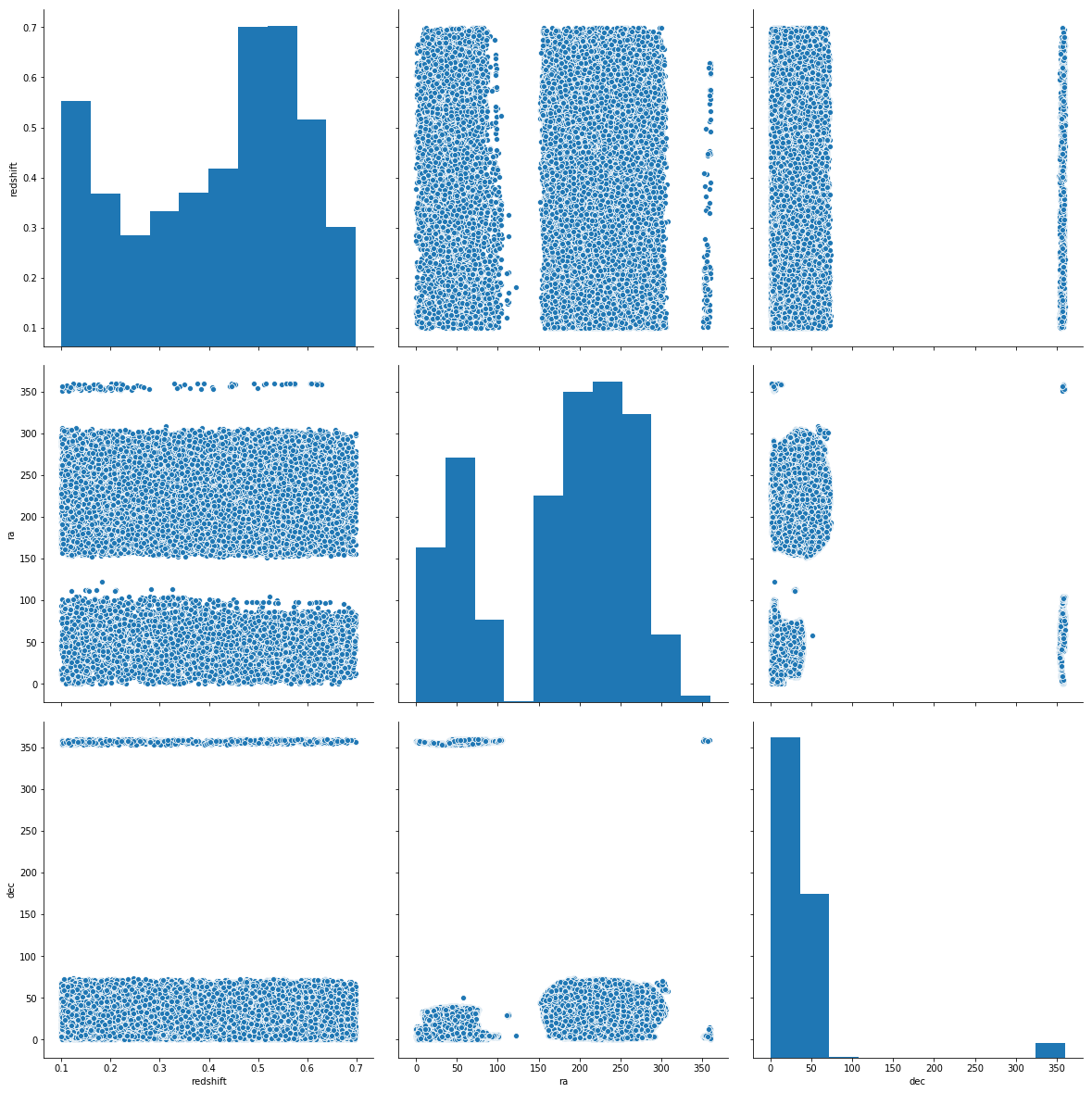
Some EDA from another notebook:
import seaborn as sns
sns.pairplot(data=df.sample(30_000), vars=['redshift', 'ra', 'dec'], height=5.5)
<seaborn.axisgrid.PairGrid at 0x7f693cebef28>
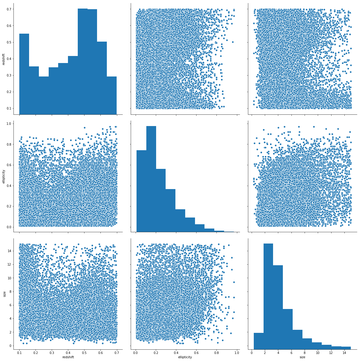
sns.pairplot(data=df.sample(30_000), vars=['redshift', 'ellipticity', 'size'], height=5.5)
<seaborn.axisgrid.PairGrid at 0x7f6939b9db38>
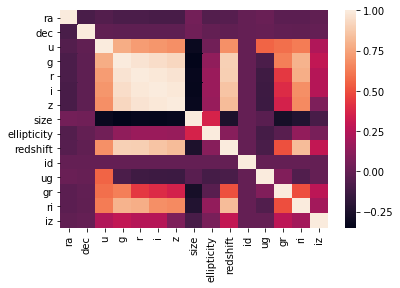
sns.heatmap(df.corr())
<matplotlib.axes._subplots.AxesSubplot at 0x7f6937e67be0>
test_df = pd.read_csv('../input/test.csv')
test_df['ug'] = test_df['u'] - test_df['g']
test_df['gr'] = test_df['g'] - test_df['r']
test_df['ri'] = test_df['r'] - test_df['i']
test_df['iz'] = test_df['i'] - test_df['z']
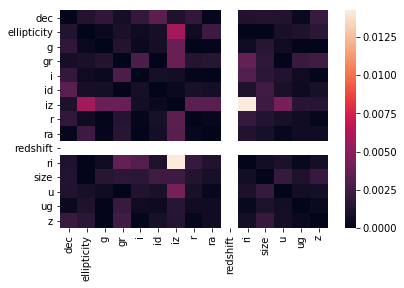
sns.heatmap(np.abs(test_df.corr() - df.corr()))
<matplotlib.axes._subplots.AxesSubplot at 0x7f6937daf198>
relevant_variables = ['u', 'g', 'r', 'i', 'z', 'gr', 'ri', 'iz'] # and maybe ellipticity
from sklearn.preprocessing import normalize

X_under = df[df['ra'] < 130].sample(150_000)
X_over = df[df['ra'] >= 130].sample(150_000)

X_train_over, X_test_over, y_train_over, y_test_over = train_test_split(
    normalize(X_over.drop(labels=['redshift', 'id'], axis=1)[relevant_variables]),
    X_over['redshift'], test_size=0.5, random_state=137)

X_train_under, X_test_under, y_train_under, y_test_under = train_test_split(
    normalize(X_under.drop(labels=['redshift', 'id'], axis=1)[relevant_variables]),
    X_under['redshift'], test_size=0.5, random_state=137)
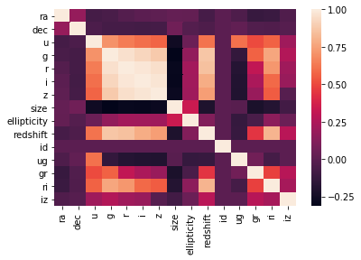
sns.heatmap(X_under.corr())
<matplotlib.axes._subplots.AxesSubplot at 0x7f6937db2160>
sns.heatmap(df.sample(500_000).corr() - df.sample(500_000).corr()) # they are pretty much the same
<matplotlib.axes._subplots.AxesSubplot at 0x7f6936c25cf8>
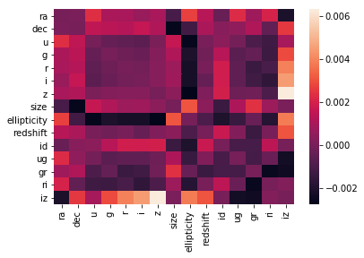
sns.heatmap(X_under.corr() - X_over.corr(), vmin=-0.1, vmax=0.1) # they are NOT
<matplotlib.axes._subplots.AxesSubplot at 0x7f6936b59dd8>
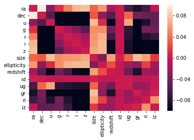
On the correlation plots above it can be seen that mainly the previously chosen relevant_variables are correletad linearly with the redshift variable.
That’s it for today. I am currently working on a Python based Keras backend API for an image preditor frontend application but Heroke doesn’t seem to like me loading a pre-trained ResNet50. I’ll also bring some advanced usage of pre-trained models on histopathologic image samples.
@Regards, Alex

Alex Olar
Christian, foodie, physicist, tech enthusiast