Almost variational autoencoders on different datasets - neuroscience (2.)

Sunday. May 05, 2019 - 14 mins

About this project

Last week I realized that I needed to collect my code and form it into a useable entity so I wrote a python package. It was not especially hard since I almost had the code completely, although I had some issues with __init__.py and setup.py files along the way but I succeeded during one of my lectures.

In this package which is freely available on pip it is possible to define and use different architectures for experimenting with autoencoders and variational autoencoders. It provides a clean interface for data handling, model building and training. You’ll be able to see how straight-forward and easy it is to use the library.

The models are built on top of the Keras API. I use dense and convolutional models that are high capacity to be able to fit different types of data efficiently.

There are some requirements for the data as of now. The package handles pickled files in 28 x 28 pixels format. I created a dataset on Kaggle which contains data in this format and well known datasets such as the CIFAR-10, dsprites, MNIST and FashionMNIST images as well as texture images from the Wigner CSNL group.

The minimum latent space capacity for the convolutional model is 16 that might change in a later version.

## 1. Testing my autoencoders on the CIFAR-10 dataset

I am still running my code on Kaggle due to its P100 Nvidia GPUs. My package can be downloaded from pip here. The latest version is 1.31dev0 as of now but I’ll be using different versions throughout this post. My code also can be found on GitHub.

!pip install csnl-vae-olaralex==0.97dev0

This command can be used on Kaggle to install a custom package and not loose GPU support.

from csnl import (DenseAutoEncoder, ConvolutionalAutoEncoder,
                  ModelTrainer, DataGenerator, VAEPlotter)

Using TensorFlow backend.

I am hosting my data on Kaggle as well so I’m reading it from there.

datagen = DataGenerator(image_shape=(28, 28, 3), batch_size=100, file_path='../input/cifar10.pkl')

Mean: 0.468, Standard Deviation: 0.247
Min: 0.000, Max: 1.000

Useful info about the data in general. The generator already expects normalized data.

dense_ae = DenseAutoEncoder(input_shape=(28*28*3,), latent_dim=512)
conv_ae = ConvolutionalAutoEncoder(input_shape=(28, 28, 3), latent_dim=512)

###
###
### Training on CIFAR-10
###
###

dense_trainer = ModelTrainer(dense_ae, datagen, loss_fn='normal', lr=1e-4, decay=5e-5)
conv_trainer = ModelTrainer(conv_ae, datagen, loss_fn='normal', lr=1e-4, decay=5e-5)

I am using normal loss and learning rate and decay can be set during the trainer class initialization. Some info about the models are printed out:

_________________________________________________________________
Layer (type)                 Output Shape              Param #   
=================================================================
input_1 (InputLayer)         (None, 2352)              0         
_________________________________________________________________
model_1 (Model)              (None, 256)               1336832   
_________________________________________________________________
dense_6 (Dense)              (None, 512)               131584    
_________________________________________________________________
model_2 (Model)              (None, 2352)              1470256   
=================================================================
Total params: 2,938,672
Trainable params: 2,938,672
Non-trainable params: 0
_________________________________________________________________
_________________________________________________________________
Layer (type)                 Output Shape              Param #   
=================================================================
input_5 (InputLayer)         (None, 28, 28, 3)         0         
_________________________________________________________________
model_5 (Model)              (None, 2048)              1120256   
_________________________________________________________________
dense_7 (Dense)              (None, 512)               1049088   
_________________________________________________________________
model_6 (Model)              (None, 28, 28, 3)         5340931   
=================================================================
Total params: 7,510,275
Trainable params: 7,510,275
Non-trainable params: 0
_________________________________________________________________

Fitting the model is very easy, only the number of epochs and the steps required as inputs.

dense_trainer.fit(1200, 250)

Epoch 1/1200
250/250 [==============================] - 4s 16ms/step - loss: 27962.8371 - val_loss: 14890.3442
Epoch 2/1200
250/250 [==============================] - 2s 7ms/step - loss: 12321.8408 - val_loss: 10661.1669
Epoch 3/1200
250/250 [==============================] - 2s 7ms/step - loss: 9898.1029 - val_loss: 9130.9680
Epoch 4/1200
250/250 [==============================] - 2s 7ms/step - loss: 8724.8514 - val_loss: 8186.6335
#####################################################################################
##################### INTENTIONALLY LEFT OUT THIS PART ##############################
#####################################################################################
Epoch 176/1200
250/250 [==============================] - 2s 7ms/step - loss: 2681.6040 - val_loss: 2680.0338
Epoch 177/1200
 73/250 [=======>......................] - ETA: 1s - loss: 2668.7087

The model is trained. For some reason Kaggle doesn’t output every line from the terminal output therefore the pretty history plot is not shown here. Moving on to training the convolutional model.

conv_trainer.fit(600, 200)

Epoch 1/600
200/200 [==============================] - 23s 113ms/step - loss: 28640.5686 - val_loss: 13880.4820
Epoch 2/600
200/200 [==============================] - 20s 98ms/step - loss: 12032.5053 - val_loss: 10606.3598
Epoch 3/600
200/200 [==============================] - 20s 98ms/step - loss: 9792.2141 - val_loss: 8963.5129
Epoch 4/600
200/200 [==============================] - 20s 98ms/step - loss: 8602.4715 - val_loss: 8253.9776
#####################################################################################
##################### INTENTIONALLY LEFT OUT THIS PART ##############################
#####################################################################################
Epoch 66/600
200/200 [==============================] - 20s 98ms/step - loss: 2158.5933 - val_loss: 2140.1205
Epoch 67/600
200/200 [==============================] - 20s 98ms/step - loss: 2144.8724 - val_loss: 2138.3434
Epoch 68/600
 97/200 [=============>................] - ETA: 9s - loss: 2123.0146

I also wrote a class to plot a grid plot and in a later version it does some random image generation from the latent space.

dense_plotter = VAEPlotter(dense_trainer, datagen)
conv_plotter = VAEPlotter(conv_trainer, datagen)

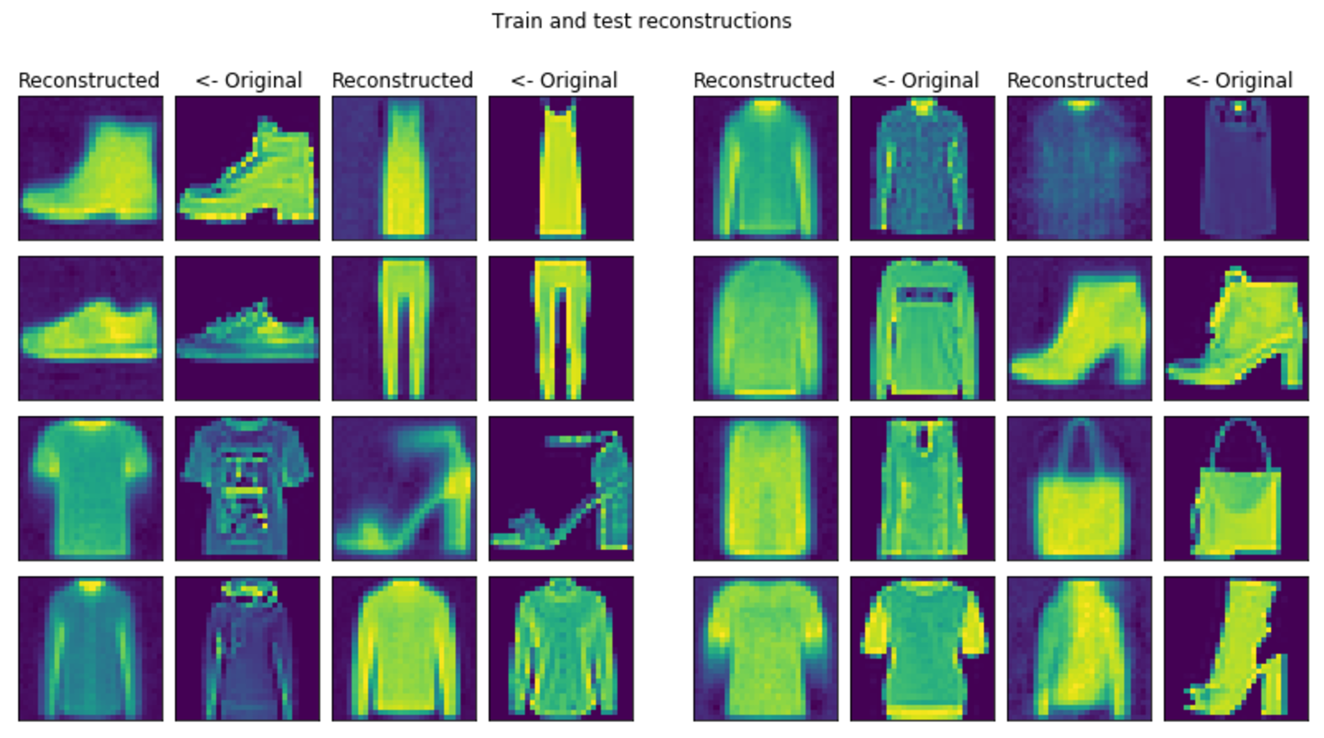
It can be seen that the outputted values are sometimes over 1 thus not perfect but the images look very similair.

dense_plotter.grid_plot()

png

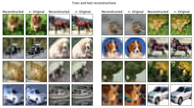
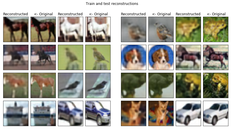
And obviously the convolutional model produces much better reconstructions.

conv_plotter.grid_plot()

png

2. Finally building variational models

I consider my autoencoders capable of fitting data properly and so I decided to finally implement variational models. Variational autoencoders differ from autoencoders by the constraints on the latent space imposed by an extra loss function. An assumed Normal-distribution is used for the latent space and it is being forced on the latent vector between encoder and decoder. For the extra additive loss KL-divergence is used which measures the difference between two probability distributions.

\[D_{KL} (P || Q) = - \sum_{x \in \chi} P(x) log\Big(\frac{Q(x)}{P(x)}\Big)\]

There are some neat tricks to do this efficently and is only made possible by those since back-propagation cannot be done on stochastic models. Read more about the reparametrization trick and its implementation by Francois Chollet on the Keras blog.

1. Testing it on the dsprites dataset

Dsprites contains figures such as circles, hearts, squares on different areas of the image. The problem is actually binary but accidentally I used a normal loss. KL divergence is not used but the model is sampled in the latent space so the expected behaviour is as good reconstruction as with autoencoders.

!pip install csnl-vae-olaralex==1.3dev0

from csnl import DenseVAE, ConvolutionalVAE, ModelTrainer, DataGenerator, VAEPlotter

Using TensorFlow backend.

textures_datagen = DataGenerator(image_shape=(28, 28, 1), batch_size=64,
                                 file_path='../input/dsprites.pkl')

Mean: 0.042, Standard Deviation: 0.202
Min: 0.000, Max: 1.000

conv_vae = ConvolutionalVAE(input_shape=(64, 28, 28, 1), latent_dim=16)

conv_trainer = ModelTrainer(conv_vae, textures_datagen, loss_fn='normal', lr=1e-4, decay=5e-5, beta=0.00)

__________________________________________________________________________________________________
Layer (type)                    Output Shape         Param #     Connected to                     
==================================================================================================
input_1 (InputLayer)            (64, 28, 28, 1)      0                                            
__________________________________________________________________________________________________
model_1 (Model)                 multiple             1116160     input_1[0][0]                    
__________________________________________________________________________________________________
dense_1 (Dense)                 (64, 16)             32784       model_1[1][0]                    
__________________________________________________________________________________________________
dense_2 (Dense)                 (64, 16)             32784       model_1[1][0]                    
__________________________________________________________________________________________________
lambda_1 (Lambda)               (64, 16)             0           dense_1[0][0]                    
                                                                 dense_2[0][0]                    
__________________________________________________________________________________________________
model_2 (Model)                 multiple             7382529     lambda_1[0][0]                   
==================================================================================================
Total params: 8,564,257
Trainable params: 8,564,257
Non-trainable params: 0
__________________________________________________________________________________________________

Only trained the convolutional model since it produces much better results.

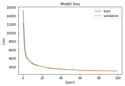
conv_trainer.fit(100, 300)

Epoch 1/100
300/300 [==============================] - 32s 105ms/step - loss: 15349.7343 - KL_divergence: 0.0000e+00 - val_loss: 12328.4790 - val_KL_divergence: 0.0000e+00
Epoch 2/100
300/300 [==============================] - 28s 93ms/step - loss: 10570.2630 - KL_divergence: 0.0000e+00 - val_loss: 7154.9893 - val_KL_divergence: 0.0000e+00
#####################################################################################
##################### INTENTIONALLY LEFT OUT THIS PART ##############################
#####################################################################################
Epoch 18/100
300/300 [==============================] - 28s 93ms/step - loss: 2195.4874 - KL_divergence: 0.0000e+00 - val_loss: 2201.9664 - val_KL_divergence: 0.0000e+00
Epoch 19/100
 64/300 [=====>........................] - ETA: 13s - loss: 2160.5529 - KL_divergence: 0.0000e+00

png

conv_plotter = VAEPlotter(conv_trainer, textures_datagen)

conv_plotter.grid_plot()

png

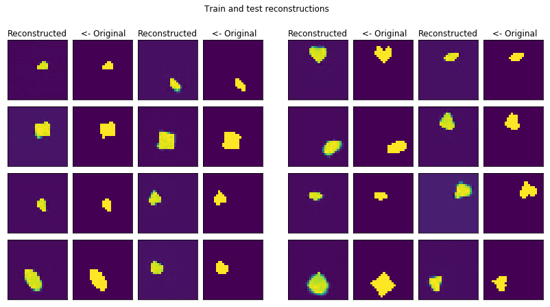
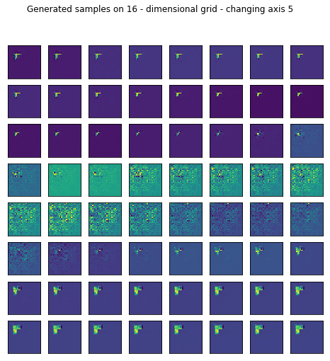
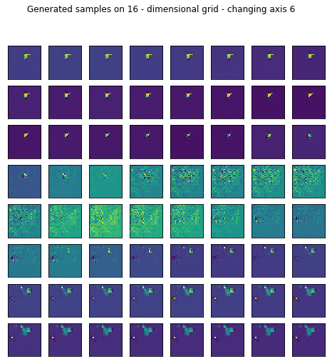
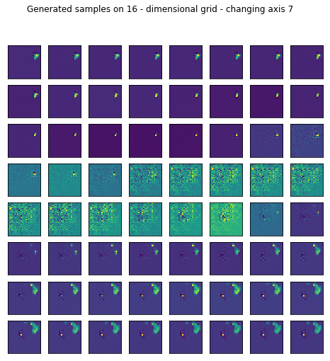
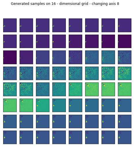
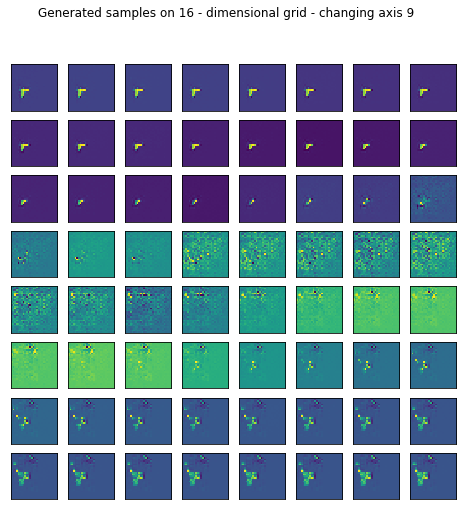
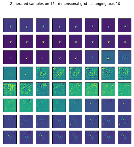
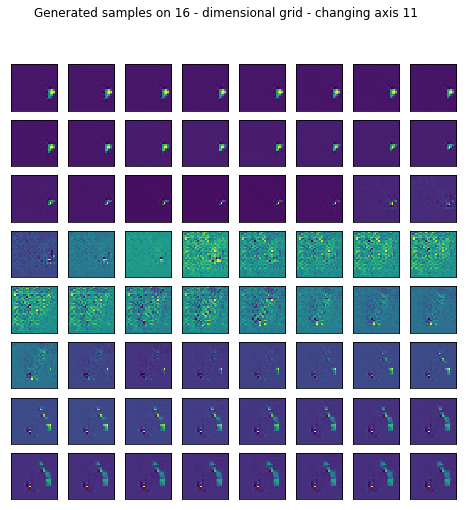
Reconstruction is pretty good but I wanted to see what happens if I generate random samples in the latent space by setting most of the values fixed and sweeping through one axis.

import numpy as np

def generate_samples(generator_model, axis=0):
    sweep = np.linspace(-10, 10, 64)
    latent_inputs = np.ones(shape=(64, 16)) * 1e-3
    latent_inputs[:, axis] = sweep 

    assert len(latent_inputs) > 63, "Latent inputs should be at least 64."
    recos = generator_model.predict(latent_inputs[:64].reshape(64, 16))

    # Output 64 images
    fig, axes = plt.subplots(8, 8, sharex=True, sharey=True, figsize=(8, 8))

    for ind, ax in enumerate(axes.flatten()):
        ax.imshow(recos[ind].reshape(28, 28))
        ax.set_xticks([])
        ax.set_yticks([])

    fig.suptitle("Generated samples on %d - dimensional grid - changing axis %d" % (16, axis))
    plt.show()

I only left the somewhat representative ones displayed.

for ax in range(16):
    generate_samples(conv_trainer.generator, axis=ax)

png

2. After all TEXTURES

There is something fundamentally hard about the textures file that was provided. Almost every dataset works except that one with the methods above. I say this because I tried to reproduce natural textures, a different dataset from the same source and that also worked fine. Let’s see the results:

I. Natural textures

textures_datagen = DataGenerator(image_shape=(28, 28, 1), batch_size=100,
                                 file_path='../input/natural_80000_28px.pkl')

Mean: 0.281, Standard Deviation: 0.383
Min: 0.000, Max: 1.000

conv_vae = ConvolutionalVAE(input_shape=(100, 28, 28, 1), latent_dim=16*16)

conv_trainer = ModelTrainer(conv_vae, textures_datagen, loss_fn='normal', lr=1e-4, decay=5e-5, beta=0.00)

conv_trainer.fit(500, 300)

Epoch 1/500
300/300 [==============================] - 29s 96ms/step - loss: 28799.9403 - KL_divergence: 0.0000e+00 - val_loss: 20407.6273 - val_KL_divergence: 0.0000e+00
Epoch 2/500
300/300 [==============================] - 25s 83ms/step - loss: 20213.8911 - KL_divergence: 0.0000e+00 - val_loss: 25120.9269 - val_KL_divergence: 0.0000e+00
#####################################################################################
##################### INTENTIONALLY LEFT OUT THIS PART ##############################
#####################################################################################
Epoch 18/500
300/300 [==============================] - 25s 83ms/step - loss: 6458.3951 - KL_divergence: 0.0000e+00 - val_loss: 5990.0586 - val_KL_divergence: 0.0000e+00
Epoch 19/500
 65/300 [=====>........................] - ETA: 18s - loss: 6381.7289 - KL_divergence: 0.0000e+00

png

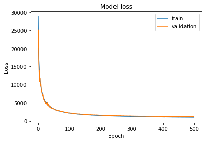
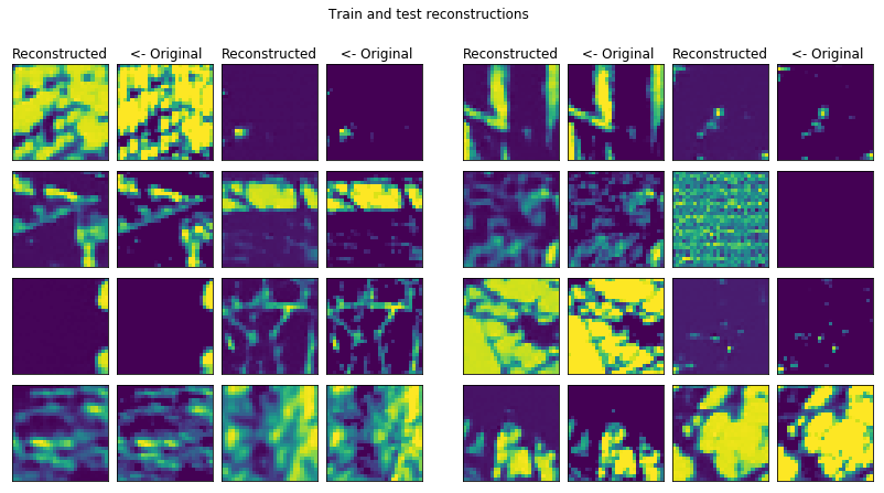
For some reason in the test set there is a seemingly totally random reconstruction. Interesting, I don’t know the reason behind yet.

II. ‘Hard’ textures

textures_datagen = DataGenerator(image_shape=(28, 28, 1), batch_size=200,
                                 file_path='../input/textures_42000_28px.pkl')

Mean: 0.499, Standard Deviation: 0.157
Min: 0.000, Max: 1.000

I assume something is fishy here since the mean of this images is 0.5 which I assume means that they are contrast normalized. Later on my task is supposed to be to learn by latent variables contrast as a latent parameter.

conv_vae = ConvolutionalVAE(input_shape=(200, 28, 28, 1), latent_dim=16*16)

conv_trainer = ModelTrainer(conv_vae, textures_datagen, loss_fn='normal', lr=1e-4, decay=5e-5, beta=0.00)

conv_trainer.fit(500, 100)

Epoch 1/500
100/100 [==============================] - 23s 226ms/step - loss: 20351.1911 - KL_divergence: 0.0000e+00 - val_loss: 15427.9461 - val_KL_divergence: 0.0000e+00
Epoch 2/500
100/100 [==============================] - 16s 161ms/step - loss: 14708.8751 - KL_divergence: 0.0000e+00 - val_loss: 14792.4794 - val_KL_divergence: 0.0000e+00
#####################################################################################
##################### INTENTIONALLY LEFT OUT THIS PART ##############################
#####################################################################################
Epoch 54/500
100/100 [==============================] - 16s 162ms/step - loss: 9705.2740 - KL_divergence: 0.0000e+00 - val_loss: 9690.3697 - val_KL_divergence: 0.0000e+00
Epoch 55/500
 65/100 [==================>...........] - ETA: 5s - loss: 9688.6837 - KL_divergence: 0.0000e+00

png

conv_plotter = VAEPlotter(conv_trainer, textures_datagen)

conv_plotter.grid_plot()

png

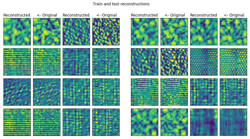
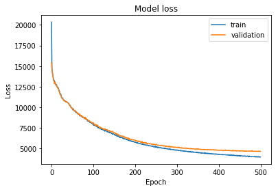
This reconstruction is the best so far I could make for this dataset. I should dive into the analysis of these pictures more in the future.

I generated some images the same way as before, now the 256 dimensional latent space was harder to sweep through but here are some randomly selected images.

png

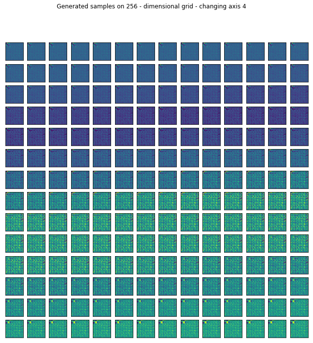
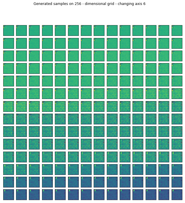
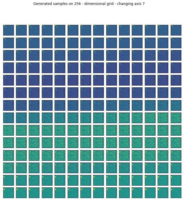
These really don’t say much about the latent representation. I’ll dive into this as well. This was it for today and the past few day’s progress. I’ll be moving on with changing the value of \(\beta\) in order to find out how it changes the latent representation by contraining it to be much more meaningful.

@Regards, Alex

Alex Olar

Christian, foodie, physicist, tech enthusiast