Variational autoencoders I.- MNIST, Fashion-MNIST, CIFAR10, textures

Intro

I have written some posts about autoencoders before and also about VAEs 1., 2. but these ones had some serious issues and I haven’t provied you with my implementation. Currently I am working on a project to build hierarchical models to better understand the visual cortex and the behaviour of V1 and V2. I’ve been through several weeks of GPU training so far and countless hours of coding and tweaking so I am going to present now what I accomplished so far.

Variational Autoencoders

I just recently found out that it wasing Kinga & Welling who first written about VAEs but it was someone else in 1995. Although it is important to mention that the first pair was able to provide a solution to backpropagation through the stochastic layer.

The main idea is that we want to do representational learning via an encoder and a decoder phase and be able to learn some form of constraint representation. We achive this by stochasticly sampling from a distribution (assume a Student-t, Gaussian, truncated Gaussian, etc.) and making the latent representation similair to it. We have this assumption since we know that the brain must encode high dimensional data in lower dimensions and also it must do so by bigger than zero activation neurons which are obviously bounded. We enforce resembalnce with the KL-divergence term in the loss function which measures the distance of two probability distributions.

Here I present a simple image of a VAE architecture which is saved from a Keras model:

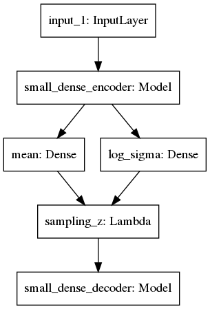
There is a clear encoding phase into mean and variance than a resampling phase from a Gaussian (or other) distribution and a decoding phase where we try to reconstruct the input image, not via learning an identity transfrom, but by learning a latent representation of the image distribution itself.

A variational autoencoder basically has three parts out of which the encoder and decoder are modular, we can simply change those to make the model bigger, smaller, constrain the encoding phase or change the architecture to convolution.

class SmallDenseVAE(VariationalAutoEncoder):

    def _encoder(self):
        input_tensor = Input(shape=self.input_shape[1:])
        x = Dense(420)(input_tensor)
        x = ReLU()(x)
        x = Dense(210)(x)
        x = ReLU()(x)
        x = Dense(105)(x)
        x = ReLU()(x)
        encoder = Model(input_tensor, x, name="small_dense_encoder")
        return encoder
    
    def _decoder(self):
        latent = Input(shape=(self.latent_dim,))
        x = Dense(200)(latent)
        x = ReLU()(x)
        x = Dense(400)(x)
        x = ReLU()(x)
        x = Dense(800)(x)
        x = ReLU()(x)
        reco = Dense(self.input_shape[1])(x)
        decoder = Model(latent, reco, name="small_dense_decoder")
        return decoder
    

The variational part is simply taking the encoded image and deriving a mean and variance than reparametrizing it to the unit-gaussian to make our later generation process easier. Some parts of the code are intentionally left out:

class VariationalAutoEncoder(Encoder):
    # Reparametrization trick
    def _sampling(self, args):
        z_mean, z_log_sigma = args
        epsilon = K.random_normal(shape=(self.BATCH_SIZE, self.latent_dim),
                                  mean=0.)
        return z_mean + K.exp(z_log_sigma) * epsilon
    
    def get_compiled_model(self, *args):
        input_img = Input(batch_shape=self.input_shape)
    
        encoder = self._encoder()
        decoder = self._decoder()
    
        encoded = encoder(input_img)
    
        # Reparametrization
        self.z_mean = Dense(self.latent_dim, name="mean")(encoded)
        self.z_log_sigma = Dense(self.latent_dim, name="log_sigma")(encoded)
        z = Lambda(self._sampling,
                   name="sampling_z")([self.z_mean, self.z_log_sigma])
    
        reco = decoder(z)
    
        model = Model(input_img, reco)
        model.beta = K.variable(self.beta)

It is possible to achive really good results with VAEs on simple datasets like MNIST, FashionMNIST or textures that I use. It is much more difficult to generate real life examples such as the CIFAR10 dataset. By good in this case I mean latent representation so sampling from the latent unit-gaussian and reconstructing the samples vector through the decoding phase. Some nice examples are presented below from trained VAE:

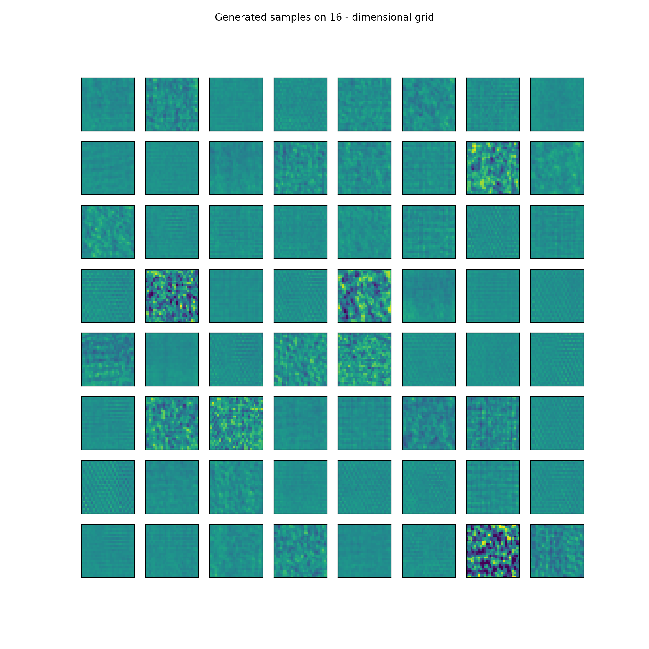
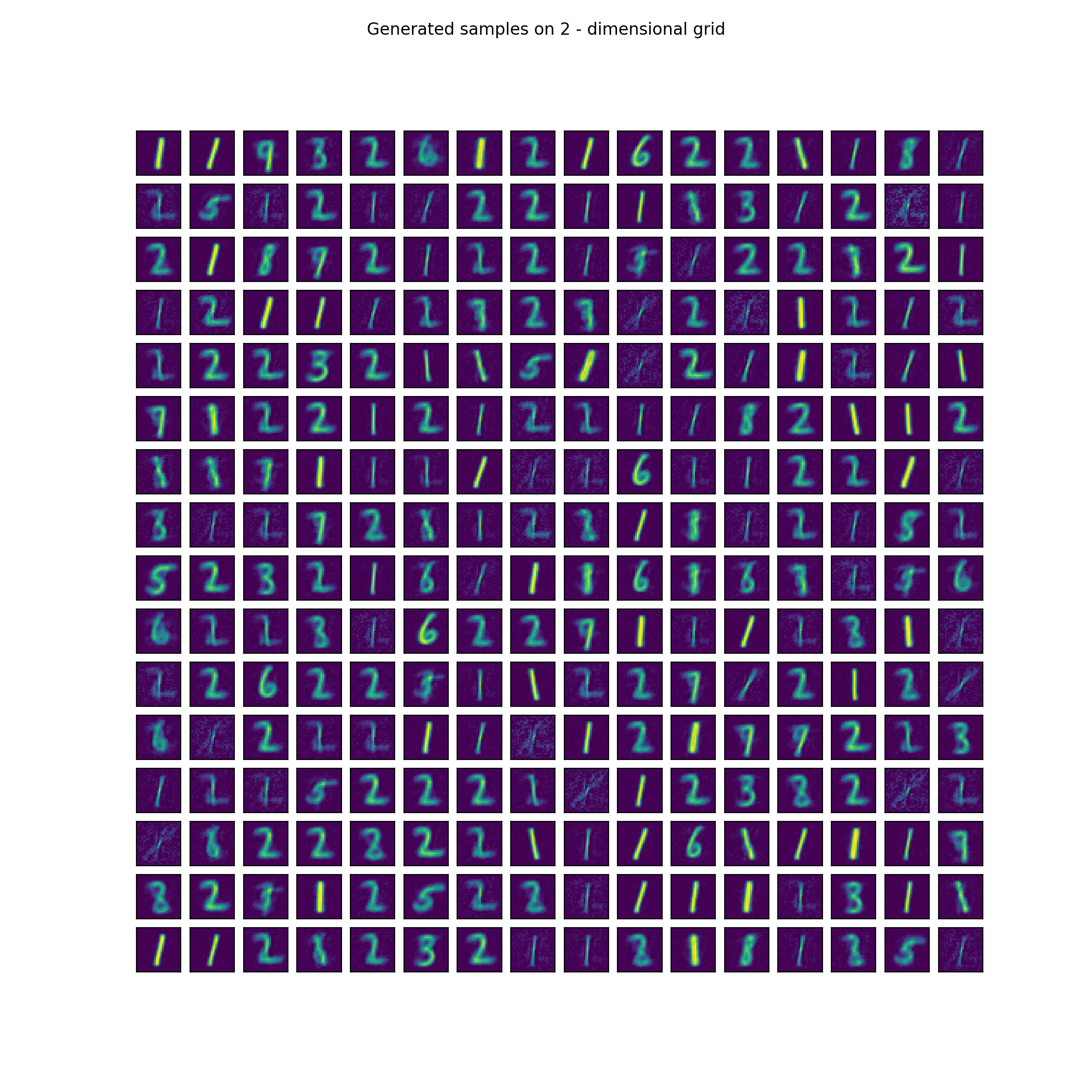
These are just random samples from 16 and 2 dimensional unit-gaussian distributions but it can be seen that they are meaningful and basically new generated samples so we can say that the underlying distribution has been learnt by the algorithm.

There are several approaches on how to generate crisper images that are harder than these datasets. If we try to model faces, house interiors such as with GANs we need much bigger and more complex models such as VQ-VAE or PixelCNN or BIVA. There is some similarity between at least two of these which is basically that they use more than one-level hierarchy and threfore they are able to present better results. I have implemented an LVAE architecture which I’ll explain in the next post to accomplish better results.

VAE-framework

I have built a Python library to build simple VAEs and train them on different datasets. I have realeased the pickled files on Kaggle that are easy to use for training.

Basically all you have to do is to setup a datagenerator:

data_gen = DataGenerator(image_shape=(28, 28, 1),
                         batch_size=100,
                         file_path=os.getcwd() + "/csnl/data/textures_42000_28px.pkl")

Define a VAE architecture to use during training:

vae = DenseVAE(input_shape=(100, 28 * 28),
               latent_dim=LATENT_DIM)

We also need to setup the trainer . Here we can define what loss function to use, set hyperparameters such as learning rate or beta that is used to weigh the KL-term in the loss.

trainer = ModelTrainer(vae,
                       data_gen,
                       loss_fn="normal",
                       lr=1e-5,
                       decay=1e-5,
                       beta=100)

Learning with beta is done with incremental values to 3/7ths of the epochs if warm_up is enabled. And train:

trainer.fit(EPOCHS=1000, steps=1000, warm_up=True)

After training the models (latent model, generator, reconstructor) are saved and some statistical tools are provided as well:

plotter = VAEPlotter(trainer, data_gen, label_data_gen=None, grid_size=16)

plotter.grid_plot()

plotter.generate_samples()

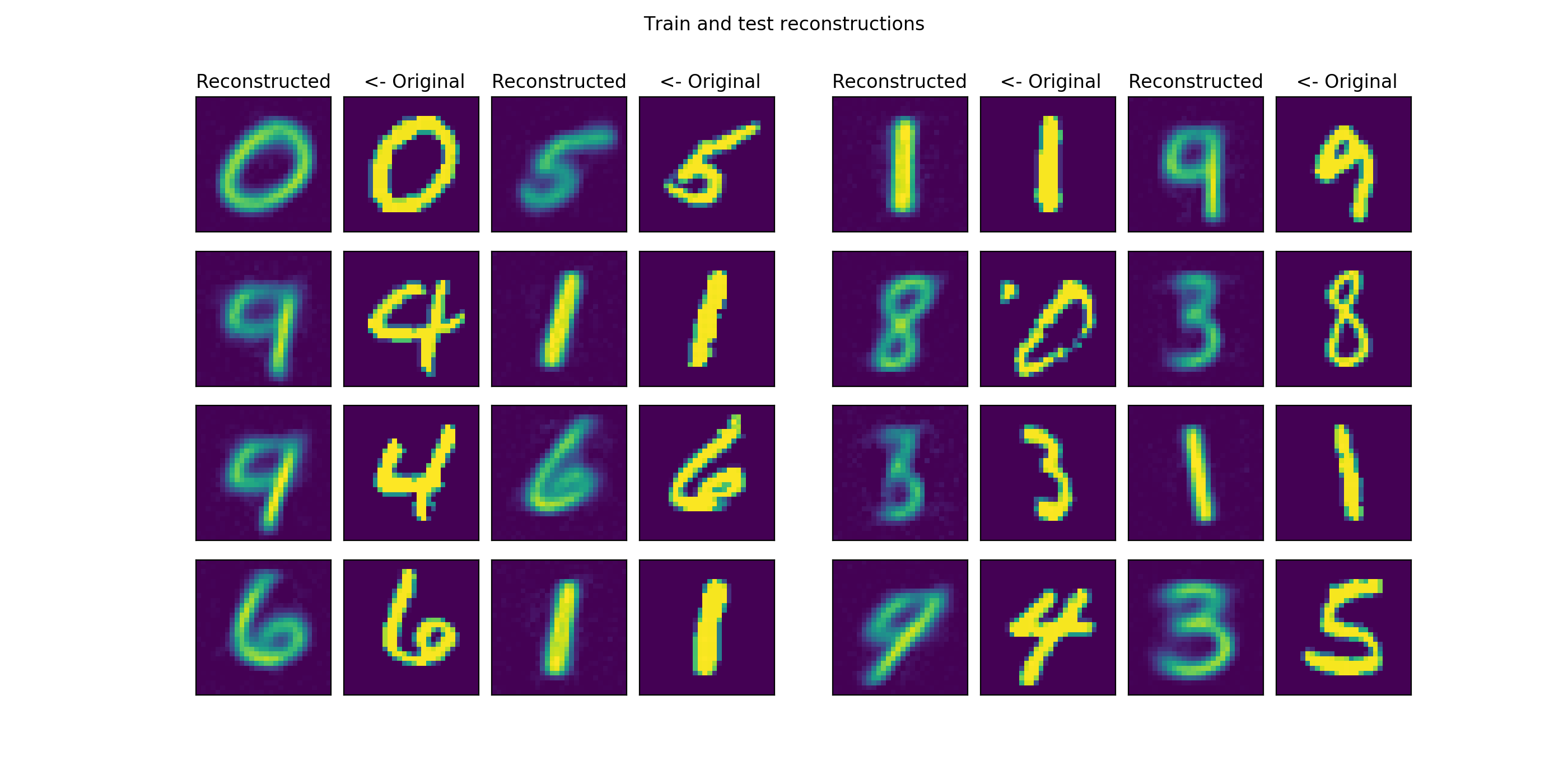
The grid_plot() method makes a plot of original and reconstructed images from the train and test sets. The generate_samples() method samples the unit-gaussian and does reconstruction through the decoder and presents results on a grid_size x grid_size grid:

The whole code base with examples runs is presented on GitHub.

@Regards, Alex

Alex Olar

Christian, foodie, physicist, tech enthusiast

Tweet Share