
Perceptron and their model with the implementation of the multi layer perceptron by hand
- 31 minsLoading the data
Titanic data, converting cabins to boolean values. It is a generally good idea to check whether a person had a cabin or not.
from sklearn.linear_model import Perceptron
%pylab inline
Populating the interactive namespace from numpy and matplotlib
import pandas as pd
data = pd.read_csv("titanic.csv")
data.head(n=10)[['Pclass', 'Sex', 'Age', 'SibSp', 'Parch', 'Fare', 'Cabin', 'Survived']]
| Pclass | Sex | Age | SibSp | Parch | Fare | Cabin | Survived | |
|---|---|---|---|---|---|---|---|---|
| 0 | 3 | male | 22.0 | 1 | 0 | 7.2500 | NaN | 0 |
| 1 | 1 | female | 38.0 | 1 | 0 | 71.2833 | C85 | 1 |
| 2 | 3 | female | 26.0 | 0 | 0 | 7.9250 | NaN | 1 |
| 3 | 1 | female | 35.0 | 1 | 0 | 53.1000 | C123 | 1 |
| 4 | 3 | male | 35.0 | 0 | 0 | 8.0500 | NaN | 0 |
| 5 | 3 | male | NaN | 0 | 0 | 8.4583 | NaN | 0 |
| 6 | 1 | male | 54.0 | 0 | 0 | 51.8625 | E46 | 0 |
| 7 | 3 | male | 2.0 | 3 | 1 | 21.0750 | NaN | 0 |
| 8 | 3 | female | 27.0 | 0 | 2 | 11.1333 | NaN | 1 |
| 9 | 2 | female | 14.0 | 1 | 0 | 30.0708 | NaN | 1 |
# Fill age with mean because only some are missing
data['Age'] = data['Age'].fillna(data['Age'].dropna().mean())
# Set NaN for Cabin to Unknown because if it would be dropped we would loose ~70% of data
data['Cabin'] = data['Cabin'].fillna('Unknown')
# For any other let's drop the record
data = data.dropna()
gender = set(data['Sex'].values)
gender = dict(zip(gender, range(len(gender))))
data['Sex'] = data['Sex'].map(lambda value: gender[value])
has_cabin = set(data['Cabin'].values)
has_cabin = dict(zip(has_cabin, range(len(has_cabin))))
data['Cabin'] = data['Cabin'].map(lambda cabin: has_cabin[cabin] != 83)
data['Cabin'] = data['Cabin'].map(lambda hasCabin: 0 if not hasCabin else 1)
data.head(n=10)[['Pclass', 'Sex', 'Age', 'SibSp', 'Parch', 'Fare', 'Cabin', 'Survived']]
| Pclass | Sex | Age | SibSp | Parch | Fare | Cabin | Survived | |
|---|---|---|---|---|---|---|---|---|
| 0 | 3 | 0 | 22.000000 | 1 | 0 | 7.2500 | 1 | 0 |
| 1 | 1 | 1 | 38.000000 | 1 | 0 | 71.2833 | 1 | 1 |
| 2 | 3 | 1 | 26.000000 | 0 | 0 | 7.9250 | 1 | 1 |
| 3 | 1 | 1 | 35.000000 | 1 | 0 | 53.1000 | 1 | 1 |
| 4 | 3 | 0 | 35.000000 | 0 | 0 | 8.0500 | 1 | 0 |
| 5 | 3 | 0 | 29.699118 | 0 | 0 | 8.4583 | 1 | 0 |
| 6 | 1 | 0 | 54.000000 | 0 | 0 | 51.8625 | 1 | 0 |
| 7 | 3 | 0 | 2.000000 | 3 | 1 | 21.0750 | 1 | 0 |
| 8 | 3 | 1 | 27.000000 | 0 | 2 | 11.1333 | 1 | 1 |
| 9 | 2 | 1 | 14.000000 | 1 | 0 | 30.0708 | 1 | 1 |
# It was shown in the previous homework that these values are the important metrics.
X = data[['Pclass', 'Sex', 'Age', 'SibSp', 'Parch', 'Fare', 'Cabin']]
y = data['Survived']
X.shape, y.shape
((889, 7), (889,))
titanic_data = X.values
titanic_data_label = y.values
Model evaluation
Using the linear perceptron with default parameters.
from sklearn.model_selection import train_test_split
from sklearn.metrics import roc_curve, roc_auc_score
def evaluate(model, X, y, test_size=0.2, fitted=False):
    X_train, X_test, y_train, y_test = train_test_split(X, y, test_size=test_size,
                                                        random_state=0, shuffle=True)
    if not fitted:
        clf = model.fit(X_train, y_train)
    else :
        clf = model

    try:
        pred_train = clf.decision_function(X_train)
        pred_test = clf.decision_function(X_test)

        plt.figure(figsize=(16, 6))
        plt.subplot(121)
        fpr, tpr, _ = roc_curve(y_train, pred_train)
        lw = 2
        plt.plot(fpr, tpr, color='darkorange',lw=lw, label="AUC = %.3f " % roc_auc_score(y_train, pred_train))
        plt.plot([0, 1], [0, 1], color='navy', lw=lw, linestyle='--')
        plt.xlim([0, 1.01])
        plt.ylim([0, 1.01])
        plt.xlabel('False Positive Rate')
        plt.ylabel('True Positive Rate')
        plt.legend(loc="lower right")
        plt.title("Training set")

        plt.subplot(122)
        fpr, tpr, _ = roc_curve(y_test, pred_test)
        lw = 2
        plt.plot(fpr, tpr, color='darkorange',lw=lw, label="AUC = %.3f " % roc_auc_score(y_test, pred_test))
        plt.plot([0, 1], [0, 1], color='navy', lw=lw, linestyle='--')
        plt.xlim([0, 1.01])
        plt.ylim([0, 1.01])
        plt.xlabel('False Positive Rate')
        plt.ylabel('True Positive Rate')
        plt.legend(loc="lower right")
        plt.title("Test set")
    except AttributeError:
        try:
            pred_train = clf.predict_proba(X_train)
            pred_test = clf.predict_proba(X_test)
        except AttributeError:
            pred_train = clf.predict(X_train)
            pred_test = clf.predict(X_test)

        plt.figure(figsize=(16, 6))
        plt.subplot(121)
        fpr, tpr, _ = roc_curve(y_train, pred_train[:, 1])
        lw = 2
        plt.plot(fpr, tpr, color='darkorange',lw=lw, label="AUC = %.3f " % roc_auc_score(y_train, pred_train[:, 1]))
        plt.plot([0, 1], [0, 1], color='navy', lw=lw, linestyle='--')
        plt.xlim([0, 1.01])
        plt.ylim([0, 1.01])
        plt.xlabel('False Positive Rate')
        plt.ylabel('True Positive Rate')
        plt.legend(loc="lower right")
        plt.title("Training set")

        plt.subplot(122)
        fpr, tpr, _ = roc_curve(y_test, pred_test[:, 1])
        lw = 2
        plt.plot(fpr, tpr, color='darkorange',lw=lw, label="AUC = %.3f " % roc_auc_score(y_test, pred_test[:, 1]))
        plt.plot([0, 1], [0, 1], color='navy', lw=lw, linestyle='--')
        plt.xlim([0, 1.01])
        plt.ylim([0, 1.01])
        plt.xlabel('False Positive Rate')
        plt.ylabel('True Positive Rate')
        plt.legend(loc="lower right")
        plt.title("Test set")

    plt.show()
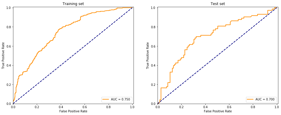
evaluate(Perceptron(), X, y)
/opt/conda/lib/python3.6/site-packages/sklearn/linear_model/stochastic_gradient.py:128: FutureWarning: max_iter and tol parameters have been added in <class 'sklearn.linear_model.perceptron.Perceptron'> in 0.19. If both are left unset, they default to max_iter=5 and tol=None. If tol is not None, max_iter defaults to max_iter=1000. From 0.21, default max_iter will be 1000, and default tol will be 1e-3.
  "and default tol will be 1e-3." % type(self), FutureWarning)
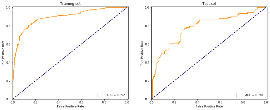
Using the multilayer perceptron to binary classify the data
from sklearn.neural_network import MLPClassifier
evaluate(MLPClassifier(), X, y)
Keras
Implementing a multilayer perceptron in keras is pretty easy since one only has to build it the layers with Sequential. One must make sure that the same parameters are used as in sklearn:
__init__(hidden_layer_sizes=(100, ), activation=’relu’, solver=’adam’, alpha=0.0001, batch_size=’auto’, learning_rate=’constant’, learning_rate_init=0.001, power_t=0.5, max_iter=200, shuffle=True, random_state=None, tol=0.0001, verbose=False, warm_start=False, momentum=0.9, nesterovs_momentum=True, early_stopping=False, validation_fraction=0.1, beta_1=0.9, beta_2=0.999, epsilon=1e-08, n_iter_no_change=10)
from keras.optimizers import SGD
from keras.models import Sequential
from keras.layers.core import Dense, Dropout, Activation
from sklearn.preprocessing import normalize
Using TensorFlow backend.
X_train, X_test, y_train, y_test = train_test_split(normalize(X.values), y.values, test_size=.2,
                                                        random_state=0, shuffle=True)
model = Sequential() # The Keras Sequential model is a linear stack of layers.
model.add(Dense(137, activation='relu', input_dim=X_train.shape[1]))
for i in range(0,6):
    model.add(Dense((420 + i*2) // 2, activation='relu'))
    if (i % 4 == 0): model.add(Dropout(0.5))
model.add(Dense(2, activation='sigmoid'))
sgd = SGD(lr=0.001, decay=0.9, momentum=0.9, nesterov=True) # Using Nesterov momentum
model.compile(loss="binary_crossentropy", optimizer='adam', metrics=["accuracy"])
print(model.summary())
_________________________________________________________________
Layer (type)                 Output Shape              Param #
=================================================================
dense_1 (Dense)              (None, 137)               1096
_________________________________________________________________
dense_2 (Dense)              (None, 210)               28980
_________________________________________________________________
dropout_1 (Dropout)          (None, 210)               0
_________________________________________________________________
dense_3 (Dense)              (None, 211)               44521
_________________________________________________________________
dense_4 (Dense)              (None, 212)               44944
_________________________________________________________________
dense_5 (Dense)              (None, 213)               45369
_________________________________________________________________
dense_6 (Dense)              (None, 214)               45796
_________________________________________________________________
dropout_2 (Dropout)          (None, 214)               0
_________________________________________________________________
dense_7 (Dense)              (None, 215)               46225
_________________________________________________________________
dense_8 (Dense)              (None, 2)                 432
=================================================================
Total params: 257,363
Trainable params: 257,363
Non-trainable params: 0
_________________________________________________________________
None
from keras.utils import to_categorical
clf = model.fit(X_train, to_categorical(y_train), epochs=10, batch_size=200,
              validation_data=(X_test, to_categorical(y_test)))
Train on 711 samples, validate on 178 samples
Epoch 1/10
711/711 [==============================] - 3s 4ms/step - loss: 0.6796 - acc: 0.5942 - val_loss: 0.6686 - val_acc: 0.5899
Epoch 2/10
711/711 [==============================] - 0s 271us/step - loss: 0.6399 - acc: 0.6245 - val_loss: 0.6790 - val_acc: 0.5899
Epoch 3/10
711/711 [==============================] - 0s 168us/step - loss: 0.6347 - acc: 0.6245 - val_loss: 0.6493 - val_acc: 0.5899
Epoch 4/10
711/711 [==============================] - 0s 126us/step - loss: 0.6191 - acc: 0.6245 - val_loss: 0.6455 - val_acc: 0.5899
Epoch 5/10
711/711 [==============================] - 0s 135us/step - loss: 0.6191 - acc: 0.6414 - val_loss: 0.6391 - val_acc: 0.6517
Epoch 6/10
711/711 [==============================] - 0s 150us/step - loss: 0.6095 - acc: 0.6857 - val_loss: 0.6486 - val_acc: 0.6517
Epoch 7/10
711/711 [==============================] - 0s 400us/step - loss: 0.6003 - acc: 0.7032 - val_loss: 0.6332 - val_acc: 0.6461
Epoch 8/10
711/711 [==============================] - 0s 138us/step - loss: 0.5996 - acc: 0.6857 - val_loss: 0.6343 - val_acc: 0.6348
Epoch 9/10
711/711 [==============================] - 0s 183us/step - loss: 0.5984 - acc: 0.6800 - val_loss: 0.6406 - val_acc: 0.6404
Epoch 10/10
711/711 [==============================] - 0s 136us/step - loss: 0.6021 - acc: 0.6864 - val_loss: 0.6341 - val_acc: 0.6489
evaluate(model, X.values, y.values, fitted=True)
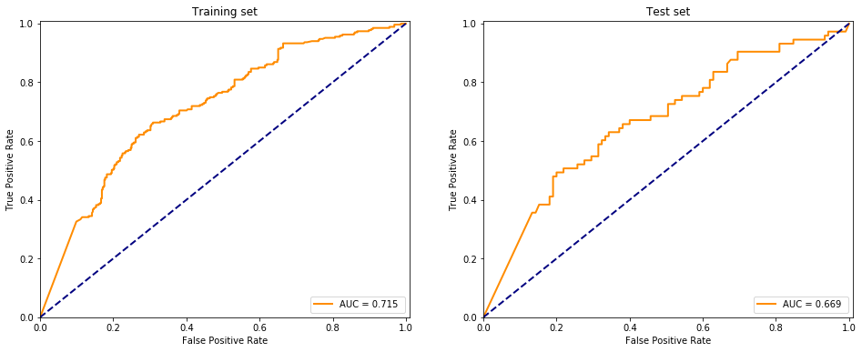
I don’t understand why but adding more layers (~100) maked the model perform worse, it is probably due to overfitting the dataset. Using a high number of neurons in the hidden layers and building up less than 10 layers the model performs somewhat accurate but not replicating the sklearn package provided MLPClassifier at all.
MNIST dataset
Training a neural network of my choice from medium.com I used a modifed version of this algorithm.
from keras.datasets import mnist
from keras.layers import Flatten
from keras.layers.convolutional import Conv2D
from keras.layers.convolutional import MaxPooling2D

(X_train, y_train), (X_test, y_test) = mnist.load_data()

X_train = normalize(X_train.reshape(X_train.shape[0], X_train.shape[1]*X_train.shape[2]))
X_test = normalize(X_test.reshape(X_test.shape[0], X_test.shape[1]*X_test.shape[2]))
X_train = X_train.reshape(X_train.shape[0], 28, 28, 1)
X_test = X_test.reshape(X_test.shape[0], 28, 28, 1)
X_train.shape, X_test.shape
((60000, 28, 28, 1), (10000, 28, 28, 1))
model = Sequential()
model.add(Conv2D(32, (5, 5), input_shape=(X_train.shape[1], X_train.shape[2], 1), activation='relu'))
model.add(MaxPooling2D(pool_size=(2, 2)))
model.add(Conv2D(32, (3, 3), activation='relu'))
model.add(MaxPooling2D(pool_size=(2, 2)))
model.add(Dropout(0.2))
model.add(Flatten())
model.add(Dense(128, activation='relu'))
model.add(Dense(10, activation='softmax'))
from keras.optimizers import Adam
model.compile(loss='categorical_crossentropy', optimizer=Adam(), metrics=['accuracy'])
model.summary()
_________________________________________________________________
Layer (type)                 Output Shape              Param #
=================================================================
conv2d_1 (Conv2D)            (None, 24, 24, 32)        832
_________________________________________________________________
max_pooling2d_1 (MaxPooling2 (None, 12, 12, 32)        0
_________________________________________________________________
conv2d_2 (Conv2D)            (None, 10, 10, 32)        9248
_________________________________________________________________
max_pooling2d_2 (MaxPooling2 (None, 5, 5, 32)          0
_________________________________________________________________
dropout_3 (Dropout)          (None, 5, 5, 32)          0
_________________________________________________________________
flatten_1 (Flatten)          (None, 800)               0
_________________________________________________________________
dense_9 (Dense)              (None, 128)               102528
_________________________________________________________________
dense_10 (Dense)             (None, 10)                1290
=================================================================
Total params: 113,898
Trainable params: 113,898
Non-trainable params: 0
_________________________________________________________________
model.fit(X_train, to_categorical(y_train),
          validation_data=(X_test, to_categorical(y_test)), epochs=10, batch_size=200)
Train on 60000 samples, validate on 10000 samples
Epoch 1/10
60000/60000 [==============================] - 27s 454us/step - loss: 0.4803 - acc: 0.8631 - val_loss: 0.1206 - val_acc: 0.9627
Epoch 2/10
60000/60000 [==============================] - 23s 375us/step - loss: 0.1117 - acc: 0.9655 - val_loss: 0.0685 - val_acc: 0.9772
Epoch 3/10
60000/60000 [==============================] - 24s 397us/step - loss: 0.0776 - acc: 0.9758 - val_loss: 0.0503 - val_acc: 0.9832
Epoch 4/10
60000/60000 [==============================] - 28s 469us/step - loss: 0.0632 - acc: 0.9802 - val_loss: 0.0463 - val_acc: 0.9857
Epoch 5/10
60000/60000 [==============================] - 28s 474us/step - loss: 0.0530 - acc: 0.9835 - val_loss: 0.0379 - val_acc: 0.9876
Epoch 6/10
60000/60000 [==============================] - 28s 474us/step - loss: 0.0461 - acc: 0.9861 - val_loss: 0.0340 - val_acc: 0.9889
Epoch 7/10
60000/60000 [==============================] - 29s 489us/step - loss: 0.0415 - acc: 0.9866 - val_loss: 0.0338 - val_acc: 0.9883
Epoch 8/10
60000/60000 [==============================] - 29s 486us/step - loss: 0.0370 - acc: 0.9883 - val_loss: 0.0294 - val_acc: 0.9909
Epoch 9/10
60000/60000 [==============================] - 27s 443us/step - loss: 0.0336 - acc: 0.9889 - val_loss: 0.0274 - val_acc: 0.9911
Epoch 10/10
60000/60000 [==============================] - 27s 456us/step - loss: 0.0309 - acc: 0.9906 - val_loss: 0.0325 - val_acc: 0.9902


<keras.callbacks.History at 0x7f1188387c50>
import itertools
from sklearn.metrics import confusion_matrix

pred_test = model.predict(X_test)

def plot_conf_matrix_of_continous_prediction(/assets/images/20181210/output):

    conf_matrix = confusion_matrix(y_test, output.argmax(axis=1), labels=range(0, 10))

    conf_matrix = normalize(conf_matrix)
    plt.figure(figsize=(10.,10.))
    plt.imshow(conf_matrix, interpolation='nearest', cmap=plt.cm.Blues)
    plt.title("Normalized confusion table of\n MNIST classification by Keras model\n")
    plt.colorbar()
    tick_marks = np.arange(10)
    plt.xticks(tick_marks, range(0, 10), rotation=60)
    plt.yticks(tick_marks, range(0, 10))
    fmt = '.5f'
    thresh = conf_matrix.max() / 2.
    for i, j in itertools.product(range(conf_matrix.shape[0]), range(conf_matrix.shape[1])):
        plt.text(j, i, format(conf_matrix[i, j], fmt), horizontalalignment="center",
                color="white" if conf_matrix[i, j] > thresh else "black")
    plt.ylabel('True label')
    plt.xlabel('Predicted label')
    plt.tight_layout()

    plt.show()
plot_conf_matrix_of_continous_prediction(pred_test)

This is extremely accurate, comparing it to a random forest with 100 trees:
from sklearn.ensemble import RandomForestClassifier
clf = RandomForestClassifier(n_estimators=100).fit(X_train.reshape(X_train.shape[0], 28*28), y_train)
pred_test = clf.predict_proba(X_test.reshape(X_test.shape[0], 28*28))
plot_conf_matrix_of_continous_prediction(pred_test)
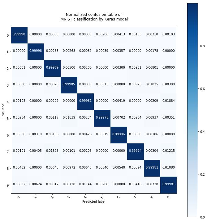
The neural network that I built with Keras according to the article seems to be better even though the random forest classifier with 100 trees is also very accurate.
Multi layer perceptron model
Implementation:
"""
    Building blocks of perceptron:
"""

def sigmoid(x):
    return 1./(1. + np.exp(-x))

def deriv_sigmoid(x):
    return sigmoid(x)*(1. - sigmoid(x))

def softmax(vec):
    return np.exp(vec)/(np.sum(np.exp(vec)) + 10**-99)
Implementation of MultiLayerPerceptron by hand with hidden layer size as parameter (name is misleading - at first I thought the naming convention was different)
class SingleLayerPerceptron:
    def __init__(self, hidden_layer_size=42, number_of_optimization_steps=75, lr=0.0001):
        self.hidden_layer_size = hidden_layer_size
        self.number_of_optimization_steps = number_of_optimization_steps
        self.lr = lr

    def fit(self, data, labels):
        self.number_of_points = data.shape[0] if data.shape[0] == labels.shape[0] else None
        self.number_of_classes = labels.shape[1]

        alpha = np.random.rand(self.hidden_layer_size, data.shape[1] + 1) # initialize regression params
        beta = np.random.rand(self.number_of_classes, self.hidden_layer_size + 1)

        for i in range(self.number_of_optimization_steps):

            vectorized_sigmoid = np.vectorize(sigmoid)

            X_with_ones = np.append(data.T, np.ones(data.shape[0]).reshape(data.shape[0], 1).T, axis=0)

            Z = np.matmul(alpha, X_with_ones)

            sigmoid_Z = vectorized_sigmoid(np.append(Z, np.ones(Z.shape[1]).reshape(1, Z.shape[1]), axis=0))

            T = np.matmul(beta, sigmoid_Z)

            T = np.array([softmax(row) for row in T.T]).T

            delta = np.multiply(T, labels.T) # K*N

            vectorized_deriv_sigmoid = np.vectorize(deriv_sigmoid)
            deriv_sigmoid_Z = vectorized_deriv_sigmoid(
                np.append(Z, np.ones(Z.shape[1]).reshape(1, Z.shape[1]), axis=0))

            s = np.multiply(deriv_sigmoid_Z, np.matmul(beta.T, delta))

            sum_delta_beta = np.matmul(delta, np.append(Z, np.ones(Z.shape[1]).reshape(1, Z.shape[1]), axis=0).T)

            sum_delta_alpha = np.matmul(s, X_with_ones.T)

            alpha = alpha - self.lr*(sum_delta_alpha[0:self.hidden_layer_size, :] + 2*alpha)
            beta = beta - self.lr*(sum_delta_beta + 2*beta)

        self.alpha = alpha
        self.beta = beta

    def predict(self, data):
        vectorized_sigmoid = np.vectorize(sigmoid)
        X_with_ones = np.append(data.T, np.ones(data.shape[0]).reshape(data.shape[0], 1).T, axis=0)
        Z = np.matmul(self.alpha, X_with_ones)
        sigmoid_Z = vectorized_sigmoid(np.append(Z, np.ones(Z.shape[1]).reshape(1, Z.shape[1]), axis=0))
        T = np.matmul(self.beta, sigmoid_Z)
        return np.array([softmax(row) for row in T.T])
data = np.random.rand(150, 3)
labels = np.random.rand(150, 2)

model = SingleLayerPerceptron()
model.fit(data, labels)

print('fitting is done')

test_data = np.random.rand(80, 3)

print(np.sum(model.predict(test_data), axis=1))
fitting is done
[1. 1. 1. 1. 1. 1. 1. 1. 1. 1. 1. 1. 1. 1. 1. 1. 1. 1. 1. 1. 1. 1. 1. 1.
 1. 1. 1. 1. 1. 1. 1. 1. 1. 1. 1. 1. 1. 1. 1. 1. 1. 1. 1. 1. 1. 1. 1. 1.
 1. 1. 1. 1. 1. 1. 1. 1. 1. 1. 1. 1. 1. 1. 1. 1. 1. 1. 1. 1. 1. 1. 1. 1.
 1. 1. 1. 1. 1. 1. 1. 1.]
from sklearn.preprocessing import normalize

X_train, X_test, y_train, y_test = train_test_split(normalize(titanic_data[0:200, :]),
                                                    to_categorical(titanic_data_label[0:200]),
                                                    test_size=0.2, random_state=0, shuffle=True)
X_train.shape, X_test.shape
((160, 7), (40, 7))
model = SingleLayerPerceptron()
model.fit(X_train, y_train)
pred_test = model.predict(X_test)
print(np.sum(pred_test, axis=1))
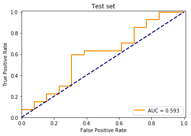
fpr, tpr, _ = roc_curve(y_test[:, 0], pred_test[:, 1])
lw = 2
plt.plot(fpr, tpr, color='darkorange',lw=lw, label="AUC = %.3f " % roc_auc_score(y_test[:, 0], pred_test[:, 1]))
plt.plot([0, 1], [0, 1], color='navy', lw=lw, linestyle='--')
plt.xlim([0, 1.01])
plt.ylim([0, 1.01])
plt.xlabel('False Positive Rate')
plt.ylabel('True Positive Rate')
plt.legend(loc="lower right")
plt.title("Test set")
plt.show()
[1. 1. 1. 1. 1. 1. 1. 1. 1. 1. 1. 1. 1. 1. 1. 1. 1. 1. 1. 1. 1. 1. 1. 1.
 1. 1. 1. 1. 1. 1. 1. 1. 1. 1. 1. 1. 1. 1. 1. 1.]
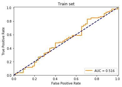
pred_train = model.predict(X_train)

print(np.sum(pred_train, axis=1))

fpr, tpr, _ = roc_curve(y_train[:, 0], pred_train[:, 1])
lw = 2
plt.plot(fpr, tpr, color='darkorange',lw=lw, label="AUC = %.3f " % roc_auc_score(y_train[:, 0], pred_train[:, 1]))
plt.plot([0, 1], [0, 1], color='navy', lw=lw, linestyle='--')
plt.xlim([0, 1.01])
plt.ylim([0, 1.01])
plt.xlabel('False Positive Rate')
plt.ylabel('True Positive Rate')
plt.legend(loc="lower right")
plt.title("Train set")
plt.show()
[1. 1. 1. 1. 1. 1. 1. 1. 1. 1. 1. 1. 1. 1. 1. 1. 1. 1. 1. 1. 1. 1. 1. 1.
 1. 1. 1. 1. 1. 1. 1. 1. 1. 1. 1. 1. 1. 1. 1. 1. 1. 1. 1. 1. 1. 1. 1. 1.
 1. 1. 1. 1. 1. 1. 1. 1. 1. 1. 1. 1. 1. 1. 1. 1. 1. 1. 1. 1. 1. 1. 1. 1.
 1. 1. 1. 1. 1. 1. 1. 1. 1. 1. 1. 1. 1. 1. 1. 1. 1. 1. 1. 1. 1. 1. 1. 1.
 1. 1. 1. 1. 1. 1. 1. 1. 1. 1. 1. 1. 1. 1. 1. 1. 1. 1. 1. 1. 1. 1. 1. 1.
 1. 1. 1. 1. 1. 1. 1. 1. 1. 1. 1. 1. 1. 1. 1. 1. 1. 1. 1. 1. 1. 1. 1. 1.
 1. 1. 1. 1. 1. 1. 1. 1. 1. 1. 1. 1. 1. 1. 1. 1.]
@Regards, Alex

Alex Olar
Christian, foodie, physicist, tech enthusiast