
T-SNE algorithm and various data related problems
- 25 mins%pylab inline
Populating the interactive namespace from numpy and matplotlib
from sklearn.manifold import TSNE
from sklearn import datasets
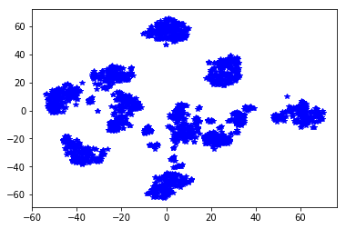
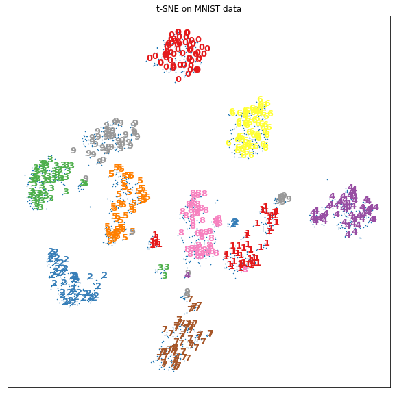
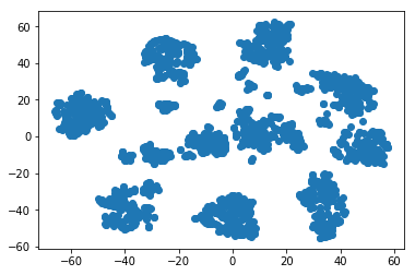
t-SNE algorithm on the MNIST dataset:
X, y = datasets.load_digits(n_class=10, return_X_y=True)
X.shape, y.shape
((1797, 64), (1797,))
X_tsne = TSNE(n_components=2,
                       init='pca',
                       random_state=42).fit_transform(X)
X_tsne.shape
(1797, 2)
plt.plot(X_tsne[:, 0], X_tsne[:, 1], 'b*')
[<matplotlib.lines.Line2D at 0x7f7b7200c7b8>]
plt.figure(figsize=(10, 10))

plt.scatter(X_tsne[:, 0], X_tsne[:, 1], marker='x', s=0.3,
           cmap=plt.cm.Set1(y/10))
for ind in range(0, X_tsne.shape[0], 3):
    plt.text(X_tsne[ind, 0], X_tsne[ind, 1], str(y[ind]),
             color=plt.cm.Set1(y[ind]/10),
            fontdict={'weight': 'bold', 'size': 13})

plt.xticks([])
plt.yticks([])
plt.title("t-SNE on MNIST data")
plt.show()
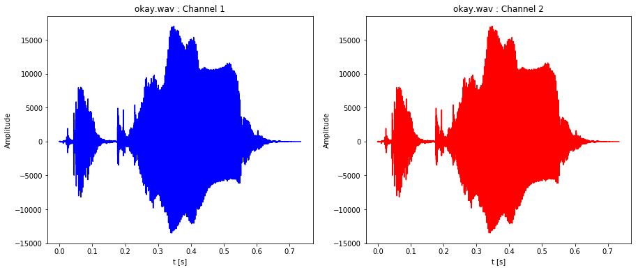
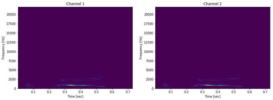
Some sound manipulation as well:
from scipy.io.wavfile import read
okay = read('okay.wav') # stereo sound with 2 channels
yes = read('yes.wav')   # but with the same values
def plot_stereo_sound_file(file_name):
    sound = read(filename=file_name)
    record_size = sound[1].shape[0]
    freq = sound[0]
    time = record_size / freq

    plt.figure(figsize=(15, 6))

    plt.subplot(121)
    plt.title(file_name + " : Channel 1")
    plt.plot(np.linspace(0, time, record_size),
             sound[1][:, 0], 'b-')
    plt.ylabel('Amplitude')
    plt.xlabel('t [s]')

    plt.subplot(122)
    plt.title(file_name + " : Channel 2")
    plt.plot(np.linspace(0, time, record_size),
             sound[1][:, 1], 'r-')
    plt.ylabel('Amplitude')
    plt.xlabel('t [s]')

    plt.show()
plot_stereo_sound_file('okay.wav')
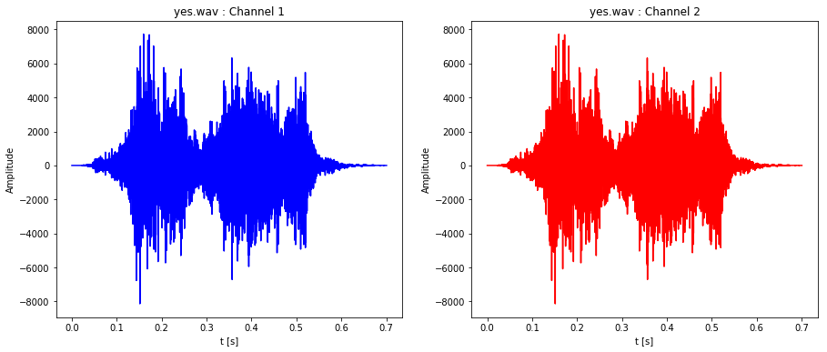
plot_stereo_sound_file('yes.wav')
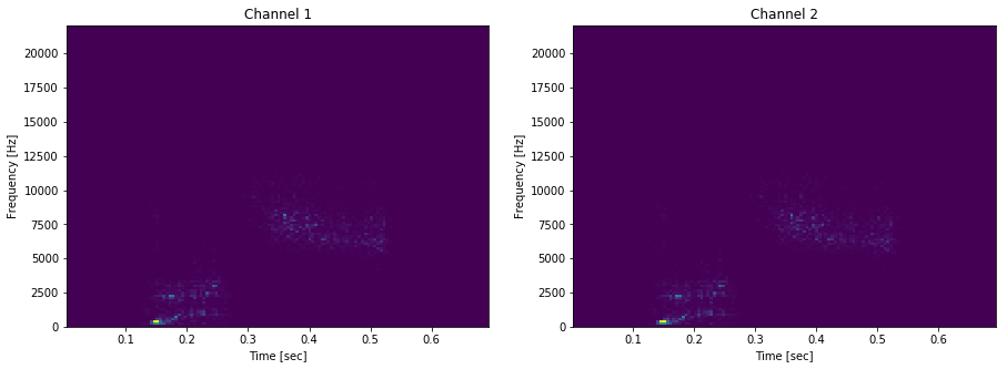
from scipy.signal import spectrogram

def plot_spectogram_of_wav_file(file_name):
    sound = read(filename=file_name)
    plt.figure(figsize=(15, 5))
    plt.subplot(121)
    plt.title('Channel 1')
    f, t, Sxx = spectrogram(sound[1][:, 0], sound[0])
    plt.pcolormesh(t, f, Sxx)
    plt.ylabel('Frequency [Hz]')
    plt.xlabel('Time [sec]')

    plt.subplot(122)
    plt.title('Channel 2')
    f, t, Sxx = spectrogram(sound[1][:, 1], sound[0])
    plt.pcolormesh(t, f, Sxx)
    plt.ylabel('Frequency [Hz]')
    plt.xlabel('Time [sec]')
    plt.show()
plot_spectogram_of_wav_file('okay.wav')
plot_spectogram_of_wav_file('yes.wav')
And of course it is part of data science to handle text as well - Twitter (!)
import re

class StringTokenizer:

    def __init__(self, text, tokenized_text=None, dictionary=None):
        self.text = text
        self.tokenized_text = None
        self.dictionary = None

    def tokenize(self, text_only=False):
        splitted_on_white_spaces = str.split(self.text)
        splitted_on_white_spaces = list(map(lambda val : val.lower(), splitted_on_white_spaces))
        splitted_on_non_alpha_as_well = []
        for splitted in splitted_on_white_spaces:
            splits = re.split('[^a-zA-Z]', splitted)
            for split in splits:
                if len(split) > 0:
                    splitted_on_non_alpha_as_well.append(split.lower())
        self.tokenized_text = splitted_on_non_alpha_as_well
        if not text_only:
            return self
        return splitted_on_non_alpha_as_well

    def build_dict(self):
        if self.tokenized_text == None:
            self = tokenize(self.text)
        distinct_words = np.array(list(set(self.tokenized_text)))
        dictionary = dict()
        for i in range(0, distinct_words.shape[0]):
            vec = [0]*distinct_words.shape[0]
            vec[i] = 1
            dictionary[distinct_words[i]] = np.array(vec)
        self.dictionary = dictionary
        return self

    def encode(self, text_to_encode):
        splitted = StringTokenizer(text_to_encode).tokenize(True)
        encoded_text = []
        for word in splitted:
            try:
                encoded_text.append(self.dictionary[word])
            except KeyError:
                encoded_text.append(word)

        return encoded_text
encoder = StringTokenizer("""Jó volna egy kicsi babszemnek lenni.

                             Vegyen körbe a héjam, mint magzatburok.
                             Egy hosszú télre, legyen ágyam feketeföld, a jó csernozjom.

                             Ne ébresszen fel se vihar, se veréb sírás, se harangszó.
                             Legyen társam a csend, a mozdulatlan, a belső való.

                             Egy kicsit ne kerüljön a helyére semmi.
                             Ne kérdezze meg senki, hogy mettől és meddig.
                             Szállingózzon a hó! Korcsolyázzanak a gyerekek! Pompázzon az újévi tűzijáték
                                 is ahogy csak akar!
                             Történjék akármi rendben vagy rendetlen odafent!

                             Minden babszem, addig hadd aludjon kicsit nyugton.

                             Tud majd repedni szépen, ahogy kell.
                             Mikor már a csíra feszíti az utat benne növekedésre.
                             A babszemek az ilyet természetesen szokták csinálni.
                             Úgy is eljön, aminek jönnie kell.""").tokenize().build_dict()
encoder.encode("Alex egy nagy babszem!")
['alex',
 array([0, 0, 0, 0, 0, 0, 0, 1, 0, 0, 0, 0, 0, 0, 0, 0, 0, 0, 0, 0, 0, 0,
        0, 0, 0, 0, 0, 0, 0, 0, 0, 0, 0, 0, 0, 0, 0, 0, 0, 0, 0, 0, 0, 0,
        0, 0, 0, 0, 0, 0, 0, 0, 0, 0, 0, 0, 0, 0, 0, 0, 0, 0, 0, 0, 0, 0,
        0, 0, 0, 0, 0, 0, 0, 0, 0, 0, 0, 0, 0, 0, 0, 0, 0, 0, 0, 0, 0, 0,
        0, 0, 0, 0, 0, 0, 0, 0, 0, 0, 0, 0, 0, 0, 0, 0, 0]),
 'nagy',
 array([0, 0, 0, 0, 0, 0, 0, 0, 0, 0, 0, 0, 0, 0, 0, 0, 0, 0, 0, 0, 0, 0,
        0, 0, 0, 0, 0, 0, 0, 0, 0, 0, 0, 0, 0, 0, 0, 0, 0, 0, 0, 0, 0, 0,
        0, 0, 0, 0, 0, 0, 0, 0, 0, 0, 0, 0, 0, 0, 0, 0, 0, 0, 0, 0, 0, 0,
        0, 0, 0, 0, 0, 0, 0, 0, 0, 0, 0, 0, 0, 0, 0, 0, 0, 0, 0, 0, 0, 0,
        0, 0, 0, 0, 0, 0, 0, 0, 1, 0, 0, 0, 0, 0, 0, 0, 0])]
Small and naive t-SNE algorithm for only 2D embedding - it did not work out well so I just copied the algorithm from the original author of the T-SNE algortihm and ran that instead, but the at least I learned about the general idea about it and the underlying matrices behind it.
X, y = datasets.load_digits(n_class=10, return_X_y=True)
X = X/255.
conditional_probability = np.ones((X.shape[0], X.shape[0]))
for i in range(X.shape[0]):
    conditional_probability[i, i] = 0.

print(conditional_probability.shape)

for ind, row in enumerate(X):
    exp_sum = np.sum([np.exp(-np.linalg.norm(row - X[index, :])**2) for index in range(X.shape[0])])
    vector = np.array([
        np.exp(-np.linalg.norm(row-X[index, :])**2)/(exp_sum - 1.)
                           for index in range(X.shape[0])])
    vector[ind] = 0.
    conditional_probability[ind, :] = np.multiply(conditional_probability[ind, :], vector)

conditional_probability
(1797, 1797)


array([[0.        , 0.0005453 , 0.0005505 , ..., 0.00055383, 0.00056383,
        0.00055661],
       [0.00054664, 0.        , 0.0005621 , ..., 0.00056422, 0.00055672,
        0.00055523],
       [0.00055311, 0.00056339, 0.        , ..., 0.00056567, 0.00055611,
        0.00056166],
       ...,
       [0.00055399, 0.000563  , 0.00056316, ..., 0.        , 0.00055902,
        0.0005687 ],
       [0.00056332, 0.00055485, 0.00055299, ..., 0.00055835, 0.        ,
        0.00056177],
       [0.00055636, 0.00055362, 0.00055876, ..., 0.00056827, 0.00056202,
        0.        ]])
X, y = datasets.load_digits(n_class=10, return_X_y=True)
y = y.astype('float')
y /= 10.

mapping_conditional_probability = np.ones((y.shape[0], y.shape[0]))
for i in range(X.shape[0]):
    mapping_conditional_probability[i, i] = 0.

for ind, row in enumerate(y):
    exp_sum = np.sum([np.exp(-np.linalg.norm(row - y[index])**2) for index in range(y.shape[0])])
    vector = np.array([
        np.exp(-np.linalg.norm(row-y[index])**2)/(exp_sum - 1.)
                           for index in range(y.shape[0])])
    vector[ind] = 0.
    mapping_conditional_probability[ind, :] = np.multiply(mapping_conditional_probability[ind, :], vector)

mapping_conditional_probability
array([[0.        , 0.00070807, 0.00068714, ..., 0.00037711, 0.00031816,
        0.00037711],
       [0.00066173, 0.        , 0.00066173, ..., 0.00040947, 0.00035243,
        0.00040947],
       [0.00061044, 0.00062903, 0.        , ..., 0.00044327, 0.00038923,
        0.00044327],
       ...,
       [0.00035288, 0.00040998, 0.0004669 , ..., 0.        , 0.00066256,
        0.00066922],
       [0.00031867, 0.00037772, 0.00043885, ..., 0.00070921, 0.        ,
        0.00070921],
       [0.00035288, 0.00040998, 0.0004669 , ..., 0.00066922, 0.00066256,
        0.        ]])
shannon_entropy = [- np.matmul(conditional_probability[:, ind], np.log2(conditional_probability[:, ind])) for ind in range(conditional_probability.shape[1])]
np.array(shannon_entropy)
1797


/opt/conda/lib/python3.6/site-packages/ipykernel_launcher.py:2: RuntimeWarning: divide by zero encountered in log2


array([nan, nan, nan, ..., nan, nan, nan])
This piece of code was acquired from Laurens Van Der Maaten the orignal creator of the t-SNE algorithm.
#
#  tsne.py
#
# Implementation of t-SNE in Python. The implementation was tested on Python
# 2.7.10, and it requires a working installation of NumPy. The implementation
# comes with an example on the MNIST dataset. In order to plot the
# results of this example, a working installation of matplotlib is required.
#
# The example can be run by executing: `ipython tsne.py`
#
#
#  Created by Laurens van der Maaten on 20-12-08.
#  Copyright (c) 2008 Tilburg University. All rights reserved.

import numpy as np
import pylab


def Hbeta(D=np.array([]), beta=1.0):
    """
        Compute the perplexity and the P-row for a specific value of the
        precision of a Gaussian distribution.
    """

    # Compute P-row and corresponding perplexity
    P = np.exp(-D.copy() * beta)
    sumP = sum(P)
    H = np.log(sumP) + beta * np.sum(D * P) / sumP
    P = P / sumP
    return H, P


def x2p(X=np.array([]), tol=1e-5, perplexity=30.0):
    """
        Performs a binary search to get P-values in such a way that each
        conditional Gaussian has the same perplexity.
    """

    # Initialize some variables
    print("Computing pairwise distances...")
    (n, d) = X.shape
    sum_X = np.sum(np.square(X), 1)
    D = np.add(np.add(-2 * np.dot(X, X.T), sum_X).T, sum_X)
    P = np.zeros((n, n))
    beta = np.ones((n, 1))
    logU = np.log(perplexity)

    # Loop over all datapoints
    for i in range(n):

        # Print progress
        if i % 500 == 0:
            print("Computing P-values for point %d of %d..." % (i, n))

        # Compute the Gaussian kernel and entropy for the current precision
        betamin = -np.inf
        betamax = np.inf
        Di = D[i, np.concatenate((np.r_[0:i], np.r_[i+1:n]))]
        (H, thisP) = Hbeta(Di, beta[i])

        # Evaluate whether the perplexity is within tolerance
        Hdiff = H - logU
        tries = 0
        while np.abs(Hdiff) > tol and tries < 50:

            # If not, increase or decrease precision
            if Hdiff > 0:
                betamin = beta[i].copy()
                if betamax == np.inf or betamax == -np.inf:
                    beta[i] = beta[i] * 2.
                else:
                    beta[i] = (beta[i] + betamax) / 2.
            else:
                betamax = beta[i].copy()
                if betamin == np.inf or betamin == -np.inf:
                    beta[i] = beta[i] / 2.
                else:
                    beta[i] = (beta[i] + betamin) / 2.

            # Recompute the values
            (H, thisP) = Hbeta(Di, beta[i])
            Hdiff = H - logU
            tries += 1

        # Set the final row of P
        P[i, np.concatenate((np.r_[0:i], np.r_[i+1:n]))] = thisP

    # Return final P-matrix
    print("Mean value of sigma: %f" % np.mean(np.sqrt(1 / beta)))
    return P


def pca(X=np.array([]), no_dims=50):
    """
        Runs PCA on the NxD array X in order to reduce its dimensionality to
        no_dims dimensions.
    """

    print("Preprocessing the data using PCA...")
    (n, d) = X.shape
    X = X - np.tile(np.mean(X, 0), (n, 1))
    (l, M) = np.linalg.eig(np.dot(X.T, X))
    Y = np.dot(X, M[:, 0:no_dims])
    return Y


def tsne(X=np.array([]), no_dims=2, initial_dims=50, perplexity=30.0):
    """
        Runs t-SNE on the dataset in the NxD array X to reduce its
        dimensionality to no_dims dimensions. The syntaxis of the function is
        `Y = tsne.tsne(X, no_dims, perplexity), where X is an NxD NumPy array.
    """

    # Check inputs
    if isinstance(no_dims, float):
        print("Error: array X should have type float.")
        return -1
    if round(no_dims) != no_dims:
        print("Error: number of dimensions should be an integer.")
        return -1

    # Initialize variables
    X = pca(X, initial_dims).real
    (n, d) = X.shape
    max_iter = 500
    initial_momentum = 0.5
    final_momentum = 0.8
    eta = 500
    min_gain = 0.01
    Y = np.random.randn(n, no_dims)
    dY = np.zeros((n, no_dims))
    iY = np.zeros((n, no_dims))
    gains = np.ones((n, no_dims))

    # Compute P-values
    P = x2p(X, 1e-5, perplexity)
    P = P + np.transpose(P)
    P = P / np.sum(P)
    P = P * 4.									# early exaggeration
    P = np.maximum(P, 1e-12)

    # Run iterations
    for iter in range(max_iter):

        # Compute pairwise affinities
        sum_Y = np.sum(np.square(Y), 1)
        num = -2. * np.dot(Y, Y.T)
        num = 1. / (1. + np.add(np.add(num, sum_Y).T, sum_Y))
        num[range(n), range(n)] = 0.
        Q = num / np.sum(num)
        Q = np.maximum(Q, 1e-12)

        # Compute gradient
        PQ = P - Q
        for i in range(n):
            dY[i, :] = np.sum(np.tile(PQ[:, i] * num[:, i], (no_dims, 1)).T * (Y[i, :] - Y), 0)

        # Perform the update
        if iter < 20:
            momentum = initial_momentum
        else:
            momentum = final_momentum
        gains = (gains + 0.2) * ((dY > 0.) != (iY > 0.)) + \
                (gains * 0.8) * ((dY > 0.) == (iY > 0.))
        gains[gains < min_gain] = min_gain
        iY = momentum * iY - eta * (gains * dY)
        Y = Y + iY
        Y = Y - np.tile(np.mean(Y, 0), (n, 1))

        # Compute current value of cost function
        if (iter + 1) % 10 == 0:
            C = np.sum(P * np.log(P / Q))
            print("Iteration %d: error is %f" % (iter + 1, C))

        # Stop lying about P-values
        if iter == 100:
            P = P / 4.

    # Return solution
    return Y


if __name__ == "__main__":
    print("Run Y = tsne.tsne(X, no_dims, perplexity) to perform t-SNE on your dataset.")
    print("Running example on ~2000 MNIST digits...")
    X, y = datasets.load_digits(n_class=10, return_X_y=True)
    X /= 255.
    Y = tsne(X, 2, 64, 20.0)
Run Y = tsne.tsne(X, no_dims, perplexity) to perform t-SNE on your dataset.
Running example on ~2000 MNIST digits...
Preprocessing the data using PCA...
Computing pairwise distances...
Computing P-values for point 0 of 1797...
Computing P-values for point 500 of 1797...
Computing P-values for point 1000 of 1797...
Computing P-values for point 1500 of 1797...
Mean value of sigma: 0.041896
Iteration 10: error is 21.556162
Iteration 20: error is 17.577109
Iteration 30: error is 15.214066
Iteration 40: error is 14.405281
Iteration 50: error is 14.148528
Iteration 60: error is 13.994236
Iteration 70: error is 13.885106
Iteration 80: error is 13.784589
Iteration 90: error is 13.701260
Iteration 100: error is 13.637046
Iteration 110: error is 1.717700
Iteration 120: error is 1.571831
Iteration 130: error is 1.444324
Iteration 140: error is 1.336456
Iteration 150: error is 1.244533
Iteration 160: error is 1.169566
Iteration 170: error is 1.109592
Iteration 180: error is 1.060985
Iteration 190: error is 1.021272
Iteration 200: error is 0.988400
Iteration 210: error is 0.961090
Iteration 220: error is 0.938207
Iteration 230: error is 0.918798
Iteration 240: error is 0.902127
Iteration 250: error is 0.887652
Iteration 260: error is 0.875066
Iteration 270: error is 0.863904
Iteration 280: error is 0.853894
Iteration 290: error is 0.844901
Iteration 300: error is 0.836766
Iteration 310: error is 0.829423
Iteration 320: error is 0.822787
Iteration 330: error is 0.816710
Iteration 340: error is 0.811131
Iteration 350: error is 0.806003
Iteration 360: error is 0.801283
Iteration 370: error is 0.796909
Iteration 380: error is 0.792848
Iteration 390: error is 0.789076
Iteration 400: error is 0.785553
Iteration 410: error is 0.782282
Iteration 420: error is 0.779231
Iteration 430: error is 0.776375
Iteration 440: error is 0.773692
Iteration 450: error is 0.771158
Iteration 460: error is 0.768772
Iteration 470: error is 0.766523
Iteration 480: error is 0.764417
Iteration 490: error is 0.762420
Iteration 500: error is 0.760515
plt.scatter(Y[:, 0], Y[:, 1])
<matplotlib.collections.PathCollection at 0x7f7b26fb7390>
@Regards, Alex

Alex Olar
Christian, foodie, physicist, tech enthusiast