
Linear methods in classification
- 31 minsLinear methods in classification
1, Load data
- (A), Download data from http://science.sciencemag.org/content/early/2018/01/17/science.aar3247
- (B), Load protein levels, and convert them to numerical values if necessary
- (C), Inspect missing values, and drop patients with missing values in protein levels
- (D), Load cancer labels
2, Logisic regression with Statsmodels
- (A), Fit a logistic regression using statsmodels to cancer/normal binary labels using protein levels as inputs
- (B), Evaluate the logloss and the accuracy of the fit.
- (C), Evaluate the ROC, and AUC of the fit.
3, Hepatocellular carcinoma
- (A), Fit a logistic regression using statsmodels to Hepatocellular carcinoma (liver cancer)/normal binary labels.
- (B), Select the 4 most significant proteins and repeat the fit.
- (C), Select the 1 most significant protein and repeat the fit.
- (D), Compare the ROC, and AUC of the fits with 4 and 1 proteins. Which would you use when screening for cancers?
- (E), Interpret the results using the wikipedia page of Hepatocellular carcinoma.
4, Cross validation
- (A), Fit logistic regression using statsmodels to cancer/normal binary labels using protein levels as inputs using 5 fold cross-validation
- (B), Calculate the mean and the std of AUC values for the 5 folds, and plot the 5 ROC curves on the same plot.
5, Sklearn
- (A), Fit a logistic regression using scikit-learn to cancer/normal binary labels using protein levels as inputs
- (B), Compare the coefficient with the statsmodels output, are they the same? If not why not?
- (C), Fit logistic regression using sklearn to cancer/normal binary labels using protein levels as inputs using 5 fold cross-validation, Calculate the mean and the std of AUC values for the 5 folds, and plot the 5 ROC curves on the same plot.
- (D), Fit linear discriminant analysis using sklearn to cancer/normal binary labels using protein levels as inputs using 5 fold cross-validation, Calculate the mean and the std of AUC values for the 5 folds, and plot the 5 ROC curves on the same plot. Is it better than logistic regression?
- (E), Fit a logistic regression using scikit-learn to the multi class problem with a different class for each cancer type and one for normals. Evaluate predictions with the confusion matrix, interpret the result matrix.
1. Loading data
%pylab inline
import pandas as pd
from sklearn import metrics as ms
Populating the interactive namespace from numpy and matplotlib
xls = pd.ExcelFile('aar3247_Cohen_SM_Tables-S1-S11.xlsx') # modified excel file
proteins = pd.read_excel(xls, 'Table S3')
protein_levels = pd.read_excel(xls, 'Table S6')
cancerTypes = pd.read_excel(xls, 'Table S11')
protein_levels.columns.values
array(['Patient ID #', 'Sample ID #', 'Tumor type', 'AJCC Stage',
       'AFP (pg/ml)', 'Angiopoietin-2 (pg/ml)', 'AXL (pg/ml)',
       'CA-125 (U/ml)', 'CA 15-3 (U/ml)', 'CA19-9 (U/ml)', 'CD44 (ng/ml)',
       'CEA (pg/ml)', 'CYFRA 21-1 (pg/ml)', 'DKK1 (ng/ml)',
       'Endoglin (pg/ml)', 'FGF2 (pg/ml)', 'Follistatin (pg/ml)',
       'Galectin-3 (ng/ml)', 'G-CSF (pg/ml)', 'GDF15 (ng/ml)',
       'HE4 (pg/ml)', 'HGF (pg/ml)', 'IL-6 (pg/ml)', 'IL-8 (pg/ml)',
       'Kallikrein-6 (pg/ml)', 'Leptin (pg/ml)', 'Mesothelin (ng/ml)',
       'Midkine (pg/ml)', 'Myeloperoxidase (ng/ml)', 'NSE (ng/ml)',
       'OPG (ng/ml)', 'OPN (pg/ml)', 'PAR (pg/ml)', 'Prolactin (pg/ml)',
       'sEGFR (pg/ml)', 'sFas (pg/ml)', 'SHBG (nM)',
       'sHER2/sEGFR2/sErbB2 (pg/ml)', 'sPECAM-1 (pg/ml)', 'TGFa (pg/ml)',
       'Thrombospondin-2 (pg/ml)', 'TIMP-1 (pg/ml)', 'TIMP-2 (pg/ml)',
       'CancerSEEK Logistic Regression Score', 'CancerSEEK Test Result'],
      dtype=object)
tumorsAndProteinLevels = np.array(['Tumor type','AFP (pg/ml)', 'Angiopoietin-2 (pg/ml)', 'AXL (pg/ml)',
        'CA-125 (U/ml)', 'CA 15-3 (U/ml)', 'CA19-9 (U/ml)', 'CD44 (ng/ml)','CEA (pg/ml)', 'CYFRA 21-1 (pg/ml)',
        'DKK1 (ng/ml)', 'Endoglin (pg/ml)', 'FGF2 (pg/ml)', 'Follistatin (pg/ml)', 'Galectin-3 (ng/ml)',
        'G-CSF (pg/ml)', 'GDF15 (ng/ml)', 'HE4 (pg/ml)', 'HGF (pg/ml)', 'IL-6 (pg/ml)', 'IL-8 (pg/ml)',
        'Kallikrein-6 (pg/ml)', 'Leptin (pg/ml)', 'Mesothelin (ng/ml)', 'Midkine (pg/ml)', 'Myeloperoxidase (ng/ml)',
        'NSE (ng/ml)', 'OPG (ng/ml)', 'OPN (pg/ml)', 'PAR (pg/ml)', 'Prolactin (pg/ml)', 'sEGFR (pg/ml)',
        'sFas (pg/ml)', 'SHBG (nM)', 'sHER2/sEGFR2/sErbB2 (pg/ml)', 'sPECAM-1 (pg/ml)', 'TGFa (pg/ml)',
        'Thrombospondin-2 (pg/ml)', 'TIMP-1 (pg/ml)', 'TIMP-2 (pg/ml)'])
# Remove * and ** values
plvls = protein_levels[tumorsAndProteinLevels].applymap(lambda x: float(x[2:]) if type(x)==str and x[0:2]=="**" else x)
plvls = plvls.applymap(lambda x: float(x[1:]) if type(x)==str and x[0:1]=="*" else x)

# Drop rows containing NaN or missing value
plvls = plvls.dropna(axis='rows')

# Extract cancer types for all the corresponding protein levels
cancer_types = np.array(list(map(lambda x: 1 if x=="Normal" else 0, plvls['Tumor type'].values)))
plvls = plvls[tumorsAndProteinLevels[1:]].values
# normalizing the data (subtracting the mean, division by standard deviation and rescaling)
from sklearn.preprocessing import normalize
plvls = normalize(plvls, axis=1)
2. Logistic regression with the Statsmodels package
import statsmodels.formula.api as sm
import statsmodels.tools as smt
from sklearn.model_selection import train_test_split
# Splitting the randomized data 20%-80%
X_train, X_test, y_train, y_test = train_test_split(
    smt.add_constant(plvls), cancer_types, test_size=0.20, random_state=42)
# Logistic model on binary cancer -> healthy or not
logistic_model = sm.Logit(y_train, X_train)
# basinhopping seems to be the best option
results = logistic_model.fit(method='basinhopping', full_output=True, disp=False)
# result summmary with quite a lot of significant values
print(results.summary())
                           Logit Regression Results
==============================================================================
Dep. Variable:                      y   No. Observations:                 1442
Model:                          Logit   Df Residuals:                     1402
Method:                           MLE   Df Model:                           39
Date:                Mon, 15 Oct 2018   Pseudo R-squ.:                  0.5260
Time:                        21:42:46   Log-Likelihood:                -469.52
converged:                       True   LL-Null:                       -990.62
                                        LLR p-value:                3.346e-193
==============================================================================
                 coef    std err          z      P>|z|      [0.025      0.975]
------------------------------------------------------------------------------
const          0.6000      1.131      0.530      0.596      -1.618       2.818
x1            -3.5770      2.088     -1.713      0.087      -7.670       0.516
x2            -5.3194      7.453     -0.714      0.475     -19.928       9.289
x3             8.2998      8.143      1.019      0.308      -7.660      24.259
x4         -1073.4014    871.421     -1.232      0.218   -2781.355     634.552
x5           135.4893    536.920      0.252      0.801    -916.855    1187.833
x6         -2660.3710    716.920     -3.711      0.000   -4065.508   -1255.234
x7           717.5979   1090.987      0.658      0.511   -1420.697    2855.892
x8           -16.3977      5.892     -2.783      0.005     -27.947      -4.849
x9           -17.9177      7.834     -2.287      0.022     -33.271      -2.564
x10           60.2152    2.7e+04      0.002      0.998   -5.28e+04    5.29e+04
x11           34.0421     11.405      2.985      0.003      11.688      56.396
x12          678.2362    153.364      4.422      0.000     377.648     978.824
x13          -27.2716     14.017     -1.946      0.052     -54.745       0.201
x14          163.1523   2113.828      0.077      0.938   -3979.874    4306.179
x15          -14.8799     36.669     -0.406      0.685     -86.750      56.990
x16          -29.5278    2.1e+04     -0.001      0.999   -4.12e+04    4.11e+04
x17           -4.1072      3.054     -1.345      0.179     -10.094       1.879
x18          -86.3493    107.532     -0.803      0.422    -297.107     124.409
x19        -2646.5090    490.893     -5.391      0.000   -3608.641   -1684.376
x20          109.3728    268.396      0.408      0.684    -416.675     635.420
x21           13.7720      3.926      3.508      0.000       6.076      21.468
x22           -0.0812      0.650     -0.125      0.901      -1.354       1.192
x23         -146.5316    675.869     -0.217      0.828   -1471.211    1178.148
x24          -16.7786     11.043     -1.519      0.129     -38.423       4.866
x25        -1014.3083    332.890     -3.047      0.002   -1666.761    -361.855
x26         1859.2179    587.054      3.167      0.002     708.613    3009.823
x27          -71.5914   1.09e+04     -0.007      0.995   -2.15e+04    2.14e+04
x28           -3.6120      0.752     -4.804      0.000      -5.086      -2.138
x29            1.2209      2.400      0.509      0.611      -3.483       5.924
x30           -4.7926      0.713     -6.723      0.000      -6.190      -3.395
x31           47.3033      8.832      5.356      0.000      29.993      64.614
x32            6.0481      3.123      1.936      0.053      -0.074      12.170
x33         -242.2809    129.592     -1.870      0.062    -496.277      11.715
x34           -7.7019      5.879     -1.310      0.190     -19.225       3.821
x35           15.2673      5.866      2.602      0.009       3.769      26.765
x36          532.4986    362.637      1.468      0.142    -178.256    1243.253
x37            0.1656      1.496      0.111      0.912      -2.767       3.098
x38           -2.8102      0.912     -3.083      0.002      -4.597      -1.023
x39            4.1496      1.068      3.887      0.000       2.057       6.242
==============================================================================
# logloss is the negative loglike function
logloss = -logistic_model.loglike(results.params)
print("Logloss :", logloss)
Logloss : 469.52213049392526
train_prediction = results.predict(X_test)
pred = train_prediction
truth = y_test
print("Accuracy %.1f%%" %
      (100.*ms.accuracy_score(truth, np.array(list(map(lambda x: 1 if x > 0.5 else 0, train_prediction))))))
Accuracy 84.2%
fpr, tpr, threshold = ms.roc_curve(truth, pred)
plt.figure(figsize=(5.,5.))
lw = 2
plt.plot(fpr, tpr, color='darkorange',lw=lw, label="AUC = %.3f " % ms.auc(fpr, tpr))
plt.plot([0, 1], [0, 1], color='navy', lw=lw, linestyle='--')
plt.xlim([0.0, 1.0])
plt.ylim([0.0, 1.0])
plt.xlabel('False Positive Rate')
plt.ylabel('True Positive Rate')
plt.legend(loc="lower right")
plt.show()

3. Hepatocellular carcinoma
# Remove * and ** values
plvls = protein_levels[tumorsAndProteinLevels].applymap(lambda x: float(x[2:]) if type(x)==str and x[0:2]=="**" else x)
plvls = plvls.applymap(lambda x: float(x[1:]) if type(x)==str and x[0:1]=="*" else x)

# Drop rows containing NaN or missing value
plvls = plvls.dropna(axis='rows')

# Extract lung cancer and healthy statistics for all the corresponding protein levels
# lung_cancers = plvls.loc[plvls['Tumor type'] == 'Lung']
# no_cancers = plvls.loc[plvls['Tumor type'] == 'Normal']

# concat dataframes
df = plvls
cancers = np.array(list(map(lambda x: 1 if x=="Liver" else 0, df['Tumor type'].values)))
plevels = normalize(df.values[:,1:])
# Splitting the randomized data 20%-80%
X_train, X_test, y_train, y_test = train_test_split(
    plevels, cancers, test_size=0.20, random_state=42)
# Logistic model on binary cancer -> healthy or not
logistic_model = sm.Logit(y_train, X_train)
# basinhopping seems to be the best option
results = logistic_model.fit(method='basinhopping', full_output=True, disp=False)
# result summmary with quite a lot of significant values
print(results.summary())
                           Logit Regression Results
==============================================================================
Dep. Variable:                      y   No. Observations:                 1442
Model:                          Logit   Df Residuals:                     1403
Method:                           MLE   Df Model:                           38
Date:                Mon, 15 Oct 2018   Pseudo R-squ.:                  0.4477
Time:                        21:42:54   Log-Likelihood:                -95.026
converged:                       True   LL-Null:                       -172.05
                                        LLR p-value:                 6.551e-16
==============================================================================
                 coef    std err          z      P>|z|      [0.025      0.975]
------------------------------------------------------------------------------
x1             3.7276      1.057      3.527      0.000       1.656       5.799
x2            -8.6690     19.760     -0.439      0.661     -47.398      30.060
x3             6.5320     29.560      0.221      0.825     -51.404      64.468
x4             6.0267    451.962      0.013      0.989    -879.802     891.856
x5            -0.6295    645.145     -0.001      0.999   -1265.090    1263.831
x6             6.6919     79.444      0.084      0.933    -149.016     162.400
x7             1.6491   4562.877      0.000      1.000   -8941.425    8944.723
x8            -1.4322      2.083     -0.687      0.492      -5.516       2.651
x9            -4.5182      5.120     -0.883      0.378     -14.553       5.516
x10            1.3307   1.17e+05   1.13e-05      1.000    -2.3e+05     2.3e+05
x11           52.0444     18.659      2.789      0.005      15.473      88.615
x12           -1.3780    668.740     -0.002      0.998   -1312.084    1309.328
x13          -66.7710     69.069     -0.967      0.334    -202.144      68.602
x14            1.6982   4602.218      0.000      1.000   -9018.483    9021.879
x15          -36.5254    119.068     -0.307      0.759    -269.895     196.844
x16            4.7640   4.67e+04      0.000      1.000   -9.16e+04    9.16e+04
x17          -45.2825     29.314     -1.545      0.122    -102.737      12.172
x18           26.4487    133.842      0.198      0.843    -235.877     288.775
x19            7.3615    587.364      0.013      0.990   -1143.850    1158.573
x20          -15.1498    219.199     -0.069      0.945    -444.772     414.472
x21            8.7405     14.674      0.596      0.551     -20.020      37.501
x22           -3.0883      1.520     -2.032      0.042      -6.067      -0.109
x23           -3.2841   3232.644     -0.001      0.999   -6339.150    6332.582
x24          -51.6663     74.528     -0.693      0.488    -197.739      94.406
x25            5.4704    488.129      0.011      0.991    -951.245     962.186
x26           -7.3590   2207.177     -0.003      0.997   -4333.347    4318.629
x27            4.1483    4.9e+04   8.46e-05      1.000   -9.61e+04    9.61e+04
x28            1.2979      0.858      1.513      0.130      -0.384       2.979
x29          -14.2841     12.416     -1.150      0.250     -38.620      10.051
x30           -0.2821      0.648     -0.435      0.663      -1.552       0.988
x31          -91.1302     49.350     -1.847      0.065    -187.854       5.593
x32            0.0814     14.340      0.006      0.995     -28.025      28.188
x33           -4.9679    782.216     -0.006      0.995   -1538.083    1528.148
x34            7.0201     19.479      0.360      0.719     -31.158      45.199
x35          -22.0093     26.141     -0.842      0.400     -73.245      29.226
x36            1.5358   2830.114      0.001      1.000   -5545.385    5548.456
x37            6.9943      2.144      3.262      0.001       2.792      11.197
x38           -1.6280      1.123     -1.450      0.147      -3.829       0.573
x39           -0.3257      3.186     -0.102      0.919      -6.571       5.919
==============================================================================

Possibly complete quasi-separation: A fraction 0.19 of observations can be
perfectly predicted. This might indicate that there is complete
quasi-separation. In this case some parameters will not be identified.
# logloss is the negative loglike function
logloss = -logistic_model.loglike(results.params)
print("Logloss :", logloss)

train_prediction = results.predict(X_test)
pred = train_prediction
truth = y_test

print("Accuracy %.1f%%" %
      (100.*ms.accuracy_score(truth, np.array(list(map(lambda x: 1 if x > 0.5 else 0, train_prediction))))))
Logloss : 95.02632456837271
Accuracy 99.2%
fpr, tpr, threshold = ms.roc_curve(truth, pred)

plt.figure(figsize=(5.,5.))
lw = 2
plt.plot(fpr, tpr, color='darkorange',lw=lw, label="AUC = %.3f " % ms.auc(fpr, tpr))
plt.plot([0, 1], [0, 1], color='navy', lw=lw, linestyle='--')
plt.xlim([0.0, 1.0])
plt.ylim([0.0, 1.0])
plt.xlabel('False Positive Rate')
plt.ylabel('True Positive Rate')
plt.legend(loc="lower right")
plt.show()
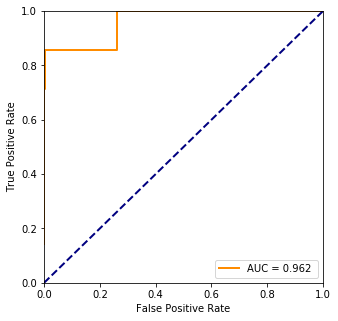
# Most significant protein levels
ind = results.pvalues.argsort()[:4]
print(ind)
sign_plevels = plevels[:, ind]
sign_plevels
[ 0 36 10 21]


array([[0.01308731, 0.18070516, 0.02382528, 0.62671162],
       [0.00297345, 0.12333307, 0.01630231, 0.88022385],
       [0.04177204, 0.05760751, 0.02306187, 0.02567324],
       ...,
       [0.00306925, 0.00209177, 0.00174422, 0.03738842],
       [0.00365565, 0.02853169, 0.0092258 , 0.02688729],
       [0.00422653, 0.06188239, 0.00841454, 0.44904901]])
The most significant value seems to be at index 0 which is the first row from plvls thus it is the AFP protein’s level. It is confirmed by the wikipedia page as well that it is an indicator of lung cancer. However, even though the accuracy of the predicted values is good, the model is not and that can be seen on the ROC curve.
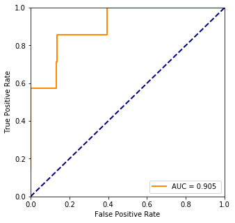
# Redoing the fit and everything

# Splitting the randomized data 20%-80%
X_train, X_test, y_train, y_test = train_test_split(
    sign_plevels, cancers, test_size=0.20, random_state=42)

# Logistic model on binary cancer -> healthy or not
logistic_model = sm.Logit(y_train, X_train)
# basinhopping seems to be the best option
results = logistic_model.fit(method='basinhopping', full_output=True, disp=False)

# result summmary with quite a lot of significant values
print(results.summary())

# logloss is the negative loglike function
logloss = -logistic_model.loglike(results.params)
print("Logloss :", logloss)

train_prediction = results.predict(X_test)
pred = train_prediction
truth = y_test

print("Accuracy %.1f%%" %
      (100.*ms.accuracy_score(truth, np.array(list(map(lambda x: 1 if x > 0.5 else 0, train_prediction))))))

fpr, tpr, threshold = ms.roc_curve(truth, pred)

plt.figure(figsize=(5.,5.))
lw = 2
plt.plot(fpr, tpr, color='darkorange',lw=lw, label="AUC = %.3f " % ms.auc(fpr, tpr))
plt.plot([0, 1], [0, 1], color='navy', lw=lw, linestyle='--')
plt.xlim([0.0, 1.0])
plt.ylim([0.0, 1.0])
plt.xlabel('False Positive Rate')
plt.ylabel('True Positive Rate')
plt.legend(loc="lower right")
plt.show()
                           Logit Regression Results
==============================================================================
Dep. Variable:                      y   No. Observations:                 1442
Model:                          Logit   Df Residuals:                     1438
Method:                           MLE   Df Model:                            3
Date:                Mon, 15 Oct 2018   Pseudo R-squ.:                 0.03755
Time:                        21:42:55   Log-Likelihood:                -165.59
converged:                       True   LL-Null:                       -172.05
                                        LLR p-value:                  0.004814
==============================================================================
                 coef    std err          z      P>|z|      [0.025      0.975]
------------------------------------------------------------------------------
x1             3.7369      0.911      4.102      0.000       1.951       5.522
x2             0.3410      2.426      0.141      0.888      -4.415       5.097
x3          -240.7636     25.488     -9.446      0.000    -290.720    -190.808
x4            -9.2729      2.208     -4.201      0.000     -13.600      -4.946
==============================================================================

Possibly complete quasi-separation: A fraction 0.18 of observations can be
perfectly predicted. This might indicate that there is complete
quasi-separation. In this case some parameters will not be identified.
Logloss : 165.58768191156673
Accuracy 98.6%
4. Cross validation
# Remove * and ** values
plvls = protein_levels[tumorsAndProteinLevels].applymap(lambda x: float(x[2:]) if type(x)==str and x[0:2]=="**" else x)
plvls = plvls.applymap(lambda x: float(x[1:]) if type(x)==str and x[0:1]=="*" else x)
# Drop rows containing NaN or missing value
plvls = plvls.dropna(axis='rows')
# Extract cancer types for all the corresponding protein levels
cancer_types = np.array(list(map(lambda x: 1 if x=="Normal" else 0, plvls['Tumor type'].values)))
plvls = plvls[tumorsAndProteinLevels[1:]].values
# Normalizing the values as well
plvls = normalize(plvls, axis=1)
# Cross validate
def cross_validate(plvls, cancer_types, k_fold=5):
logloss = []
accuracy = []
fpr = dict()
tpr = dict()
auc = []
for i in range(k_fold):
# Splitting the randomized data 20%-80%
X_train, X_test, y_train, y_test = train_test_split(plvls, cancer_types,
test_size=1./k_fold,
random_state=42*i + (137-i)*k_fold)
# Logistic model on binary cancer -> healthy or not
logistic_model = sm.Logit(y_train, X_train)
# basinhopping seems to be the best option
results = logistic_model.fit(method='basinhopping', full_output=True, disp=False)
# logloss is the negative loglike function
logloss.append(-logistic_model.loglike(results.params))
train_prediction = results.predict(X_test)
pred = train_prediction
truth = y_test
accuracy.append(100.*ms.accuracy_score(truth, np.array(list(map(lambda x: 1 if x > 0.5 else 0, train_prediction)))))
fpr[i], tpr[i], threshold = ms.roc_curve(truth, pred)
auc.append(ms.auc(fpr[i], tpr[i]))
return logloss, accuracy, auc, fpr, tpr
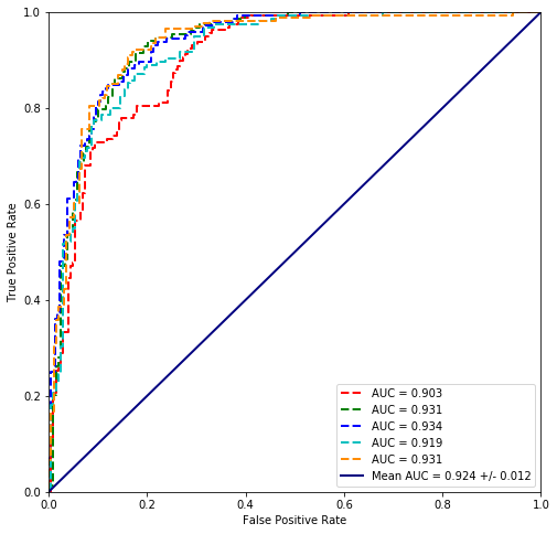
def plot_cross_validated_data(values, k_fold=5):
logloss, accuracy, auc, fpr, tpr = values
print("Mean Accuracy = %.1f%%" % np.mean(accuracy))
if(len(logloss) > 0):
print("\t\t Mean logloss = %.3f" % np.mean(logloss))
plt.figure(figsize=(8.,8.))
lw = 2
cmap = ['r', 'g', 'b', 'c', 'darkorange']
for i in range(k_fold):
plt.plot(fpr[i], tpr[i], color=cmap[i%5],lw=lw, linestyle='--', label="AUC = %.3f " % auc[i])
plt.plot([0, 1], [0, 1], color='navy', lw=lw, linestyle='-', label="Mean AUC = %.3f +/- %.3f" %
(np.mean(auc), np.std(auc)))
plt.xlim([0.0, 1.0])
plt.ylim([0.0, 1.0])
plt.xlabel('False Positive Rate')
plt.ylabel('True Positive Rate')
plt.legend(loc="lower right")
plt.show()
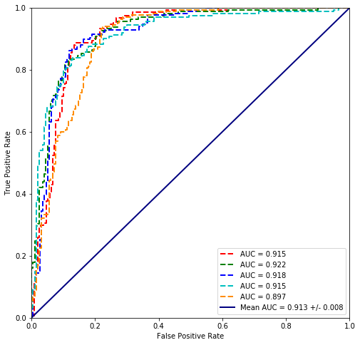
values = cross_validate(plvls, cancer_types)
plot_cross_validated_data(values)
Mean Accuracy = 85.1%
		 Mean logloss = 470.434
5. Scikit comparison
from sklearn.linear_model import LogisticRegression
# Splitting the randomized data 20%-80%
X_train, X_test, y_train, y_test = train_test_split(plvls, cancer_types,
                                            test_size=0.2, random_state=42)

clf = LogisticRegression(random_state=137, solver='lbfgs').fit(X_train, y_train)
clf.coef_
array([[-9.48707744e-01,  1.83903929e-02,  7.95491459e-01,
        -2.52954480e-02,  3.05955892e-04, -7.56440297e-02,
         9.15254779e-03, -2.67799468e+00, -8.16559492e-01,
         6.23163704e-04,  9.88404739e-01,  4.74152986e-02,
         1.17032345e-01,  7.70760276e-04, -9.34918494e-03,
        -3.84480629e-04, -7.18391518e-01, -9.01026951e-02,
        -3.18421447e-02, -7.51784431e-03,  2.11467676e+00,
         1.16728461e+00,  1.90117408e-03, -3.44293734e-01,
        -2.54546830e-02,  1.85846906e-02, -2.52367752e-04,
        -2.46246869e+00,  1.74366466e+00, -2.97473230e+00,
         2.01660531e+00,  1.33148112e+00,  9.52140907e-04,
         1.83475532e+00,  2.70761855e+00,  1.27181348e-02,
         2.10712966e-01, -7.35910282e-01,  5.88527779e+00]])
smclf = sm.Logit(y_train, X_train).fit(method='basinhopping', full_output=True, disp=False)
smclf.params
array([-3.22387768e+00, -4.82459242e+00,  8.47257625e+00, -1.07291690e+03,
        1.43809357e+02, -2.64476560e+03,  7.15330113e+02, -1.65885994e+01,
       -1.79806999e+01,  5.33958704e+01,  3.35214507e+01,  6.72095874e+02,
       -2.67618774e+01,  1.62104363e+02, -1.28811089e+01, -2.54467653e+01,
       -3.85213260e+00, -9.54969343e+01, -2.63774649e+03,  1.19648533e+02,
        1.37009167e+01,  2.31513267e-01, -1.39479210e+02, -1.73462433e+01,
       -1.01227642e+03,  1.86133386e+03, -6.88544270e+01, -3.27699019e+00,
        1.23930995e+00, -4.50896105e+00,  4.67843272e+01,  6.10458336e+00,
       -2.48495710e+02, -7.98193338e+00,  1.55007443e+01,  5.25445783e+02,
        3.22225689e-01, -2.42487203e+00,  4.41508794e+00])
They differ so maybe the problem doesn’t have one solution or doesn’t have one best solution. Also the methods with which they are looking for a solution differ as well. (Update: it turned out that they differ because scikit learn is using regulization by default. )
# Cross validate
def scikit_cross_validate(model, plvls, cancer_types, k_fold=5):
    logloss = []
    accuracy = []
    fpr = dict()
    tpr = dict()
    auc = []
    for i in range(k_fold):
        # Splitting the randomized data 20%-80%
        X_train, X_test, y_train, y_test = train_test_split(plvls, cancer_types,
                                                            test_size=1./k_fold,
                                                            random_state=137*i + i*42, shuffle=True)

        # Logistic model on binary cancer -> healthy or not
        clf = model.fit(X_train, y_train)

        train_prediction = clf.predict(X_test)
        pred_value = clf.decision_function(X_test)
        pred = train_prediction
        truth = y_test

        accuracy.append(100.*ms.accuracy_score(truth, train_prediction))

        fpr[i], tpr[i], threshold = ms.roc_curve(truth,  pred_value)

        auc.append(ms.auc(fpr[i], tpr[i]))

    return logloss, accuracy, auc, fpr, tpr
values = scikit_cross_validate(LogisticRegression(random_state=42, solver='newton-cg'), plvls, cancer_types)
plot_cross_validated_data(values)
Mean Accuracy = 79.3%
The results with scikit are ‘worse’ however the minimization method is different so Statsmodels and Scikit must get different solutions.
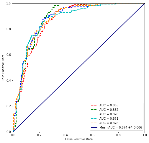
from sklearn.discriminant_analysis import LinearDiscriminantAnalysis
values = scikit_cross_validate(LinearDiscriminantAnalysis(), plvls, cancer_types)
plot_cross_validated_data(values)
Mean Accuracy = 84.0%
Linear discriminant analysis seems to fit the data best so far.
# Remove * and ** values
plvls = protein_levels[tumorsAndProteinLevels].applymap(lambda x: float(x[2:]) if type(x)==str and x[0:2]=="**" else x)
plvls = plvls.applymap(lambda x: float(x[1:]) if type(x)==str and x[0:1]=="*" else x)

# Drop rows containing NaN or missing value
plvls = plvls.dropna(axis='rows')

# Extract cancer types for all the corresponding protein levels
cancer_types = plvls['Tumor type'].values
plvls = plvls[tumorsAndProteinLevels[1:]].values

# Splitting the randomized data 20%-80%
X_train, X_test, y_train, y_test = train_test_split(plvls, cancer_types,
                                            test_size=0.2, random_state=42)

clf = LogisticRegression(random_state=137, solver='lbfgs', multi_class='multinomial').fit(X_train, y_train)
pred = clf.predict(X_test)
conf_matrix = ms.confusion_matrix(y_test, pred, labels=clf.classes_)
conf_matrix
array([[ 12,  11,   0,   0,   0,  22,   1,   3,   0],
       [  3,  43,   0,   0,   4,  16,   1,   0,   2],
       [  0,  10,   1,   0,   0,   3,   0,   1,   0],
       [  0,   1,   0,   4,   0,   0,   0,   1,   1],
       [  1,  10,   0,   0,   4,   4,   0,   1,   0],
       [  3,   5,   0,   0,   1, 148,   0,   0,   1],
       [  0,   4,   0,   0,   1,   1,   3,   0,   1],
       [  0,   3,   0,   0,   0,  15,   1,   2,   0],
       [  2,   7,   0,   0,   0,   1,   0,   0,   2]])
import itertools

conf_matrix = normalize(conf_matrix)
plt.figure(figsize=(10.,10.))
plt.imshow(conf_matrix, interpolation='nearest', cmap=plt.cm.Blues)
plt.title("Normalized confusion table of\n multinomial logistic regression model\n")
plt.colorbar()
tick_marks = np.arange(clf.classes_.size)
plt.xticks(tick_marks, clf.classes_, rotation=60)
plt.yticks(tick_marks, clf.classes_)
fmt = '.2f'
thresh = conf_matrix.max() / 2.
for i, j in itertools.product(range(conf_matrix.shape[0]), range(conf_matrix.shape[1])):
    plt.text(j, i, format(conf_matrix[i, j], fmt), horizontalalignment="center",
            color="white" if conf_matrix[i, j] > thresh else "black")
plt.ylabel('True label')
plt.xlabel('Predicted label')
plt.tight_layout()
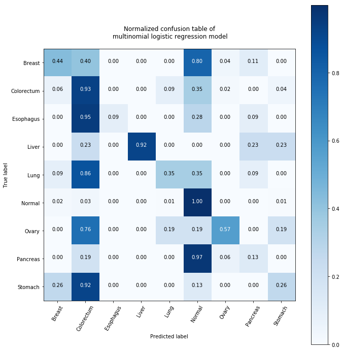
What we can learn from this? It is clear that our prediction is not that good. We predicted most of the healthy people helathy but we predicted most of the patients with Pancreas cancer healthy. Not only could we not figure out too well the cancers but also the model categorized most of cancers as Colorectum, however, I must mention that most of cancers is indeed colorectum so our model is not a complete failure.
It is also intersting that the model was capeable of identifying breast and ovary cancer pretty well and even liver cancer was identified quiet well.
@Regards, Alex

Alex Olar
Christian, foodie, physicist, tech enthusiast