Photometric redshift estimation 2.

import pandas as pd
import numpy as np
import matplotlib.pyplot as plt
%matplotlib inline
from itertools import combinations as comb
from matplotlib.patches import Patch

file = "SDSSDR7-5-percent-err-limit-10000-line"
dataset = pd.read_csv(file+".csv")
print(dataset.columns.values)

beck_columns = ['m_r', 'ug', 'gr', 'ri', 'iz'] # 5 dimensions

# Creating training and test sets from data
mask = np.random.rand(len(dataset)) < 0.8 # make the test set more then 20% of the dataset
# Convert masked data to np array
train = dataset[~mask]
test = dataset[mask]

print(train.shape, test.shape)

from sklearn.neighbors import NearestNeighbors
from sklearn.linear_model import LinearRegression

# Linear fitter for the provided training set
def linfit(x_train, y_train):
    reg = LinearRegression()
    fit = reg.fit(x_train, y_train)
    return reg

# Predict redshift based on a linear model
def predict_redshift(x_train, y_train, y_test):
    reg = linfit(x_train, y_train)
    return reg.predict(y_test.reshape(1,-1))

# Remove outliers
def calc_excluded_indices(x_reg, y_reg, k):
    deltas = []
    linreg = linfit(x_reg, y_reg)
    y_pred = linreg.predict(x_reg)
    delta_y_pred = np.sqrt(np.sum(np.square(y_reg-y_pred))/k)
    for ind in range(y_reg.size):
        err = np.linalg.norm(y_reg[ind] - y_pred[ind])
        if 3*delta_y_pred < err:
            deltas.append(ind)
    return deltas

# Subtract mean and divide by standard deviation to get 0 mean and 1 standard deviation
def normalize_dataframe(data, labels):
    df = data[labels].subtract(data[labels].mean(axis=1), axis=0)
    return df.divide(df.std(axis=1), axis=0)

def beck_method(test, train, labels, k=100):
    prediction = []
    # Normalize dataframes, test and train for appropiate labels
    df = normalize_dataframe(train, labels)
    test_df = normalize_dataframe(test, labels)
    # Fit the training data
    neigh = NearestNeighbors(n_neighbors=k, algorithm='kd_tree')
    neigh.fit(df.values)
    # Do the prediction
    for point in test_df.values:
        indices = neigh.kneighbors([point], return_distance=False)[0,:]
        redshift = predict_redshift(df.values[indices], train['z'].values[indices], point)
        # Calculate excluded indices
        deltas = calc_excluded_indices(df.values[indices], train['z'].values[indices], k)
        #Redo fit
        prev_size = indices.size
        indices = np.delete(indices, deltas)
        if indices.size < prev_size:
            redshift = predict_redshift(df.values[indices], train['z'].values[indices], point)
        prediction.append(redshift)
    return np.array(prediction)

# Make a prediction using k nearest neighbors
pred = beck_method(test, train, beck_columns, k=166)

y_test = test['z'].values
y_test = y_test.reshape(y_test.size, 1)

# Calculating the MSE
MSE = np.sum(np.square(pred-y_test))/pred.size

# Showing the prediction accuracy
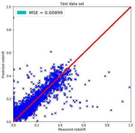
plt.figure(figsize=(7.,7.))
plt.scatter(test['z'].values, pred, marker='x', c='b')
plt.xlim(0,1)
plt.ylim(0,1)
lin = np.linspace(0,1,300)
plt.plot(lin, lin, 'r.')
plt.title('Test data set')
plt.xlabel('Measured redshift')
plt.ylabel('Predicted redshift')
legend_handle = [Patch(facecolor='c', edgecolor='c',
                         label=('MSE = %.5f' % MSE) )]
plt.legend(handles=legend_handle, loc='upper left', fontsize='x-large')
# Saving to file
plt.savefig(file+".png", dpi=166)

# Calculating the errors
y_train = y_test
errs = np.abs(pred-y_train.reshape(y_train.shape[0], 1))/y_train.shape[0]
sigma = np.std(errs)
y_train = y_train.reshape(y_train.shape[0], 1)

non_outliers = []
outliers = []
for ind in range(0, errs.size):
    if errs[ind] < 3*sigma:
        non_outliers.append(ind)
    else:
        outliers.append(ind)

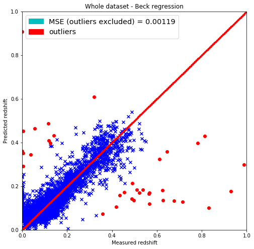
# Plotting the results
plt.figure(figsize=(8.,8.))

# Removing outliers from both predicted_redshift, and y_train sets
predicted_redshift_og = pred
predicted_redshift = predicted_redshift_og[non_outliers]
outlier_redshift = predicted_redshift_og[outliers]
# Same for measured redshifts
y_train_og = y_train
y_train = y_train_og[non_outliers]
outlier_y = y_train_og[outliers]

# Getting the mean squared error
MSE = np.sum(np.square(predicted_redshift-y_train))/y_train.shape[0]

plt.scatter(y_train, predicted_redshift, c='b', marker='x')
plt.scatter(outlier_y, outlier_redshift, c='r', marker='o')
plt.xlim(0,1)
plt.ylim(0,1)
lin = np.linspace(0,1,300)
plt.scatter(lin, lin, c='r', marker='.')
plt.title('Whole dataset - Beck regression')
plt.xlabel('Measured redshift')
plt.ylabel('Predicted redshift')
legend_handle = [Patch(facecolor='c', edgecolor='c',
                         label=('MSE (outliers excluded) = %.5f' % MSE)),
                Patch(facecolor='r', edgecolor='r',
                         label=('outliers'))]
plt.legend(handles=legend_handle, loc='upper left', fontsize='x-large')
plt.savefig(file+"-without-outliers.png", dpi=166)

import time
from sklearn.model_selection import train_test_split

def cross_validate(algo, dataset, labels, splits=5, k=10):
    MAEs = []
    MSEs = []
    start = time.time()
    for i in range(splits):
        train, test = train_test_split(dataset,
                            test_size=(1.-1./splits),
                            random_state=42*(k-i)+i*137)
        y_test = test['z'].values
        pred = algo(test, train, labels, k)
        y_test = y_test.reshape(y_test.size, 1)
        # Calculating the MAE and MSE
        MAE = np.sum(np.abs(pred-y_test))/pred.size
        MSE = np.sum(np.square(pred-y_test))/pred.size
        MAEs.append(MAE)
        MSEs.append(MSE)
    print("Mean MAE : %.5f" % np.mean(MAEs))
    print("\tStandard deviation of MAE : %.5f" % np.std(MAEs))
    print("Mean MSE : %.5f" % np.mean(MSEs))
    print("\tStandard deviation of MSE : %.5f" % np.std(MSEs))
    end = time.time()
    print("The operation took %.2f seconds.\n\n" % (end-start))

cross_validate(beck_method, dataset, beck_columns, splits=5, k=100)