
Photometric redshift estimation with statsmodels, scikit-learn and naive linear regression implementation using numpy
- 39 mins03. Lab exercises, Linear regression
1 Implement linear regression using SVD. (use np.linalg.svd). Write a class for linear regression, using the following template:
class LinReg():
    """Linear regression class."""

    def __init__(self):
        """Intialize linear regression."""
        self.coefficients = None

    def fit(self,x_train, y_train):
        """Fit linear regression."""
        return self

    def predict(self,x_test):
        """Predict with linear regression."""
        return y_test
2 Application:
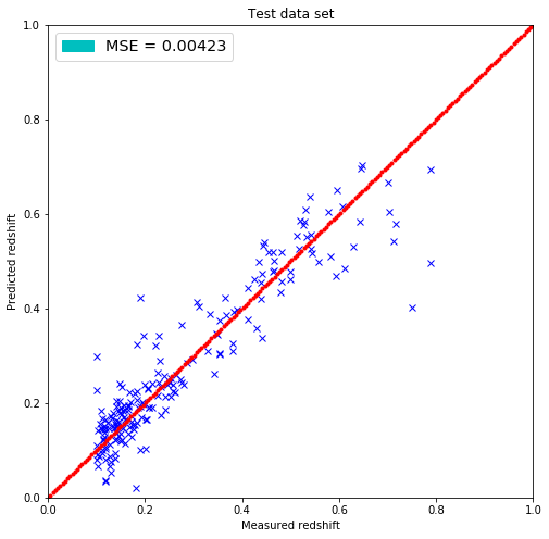
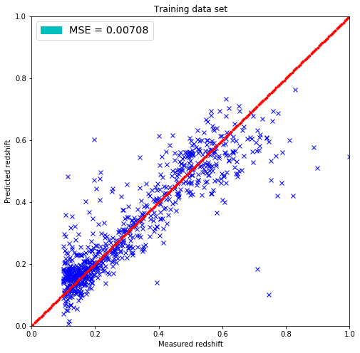
- A, Apply the linear regressor on photometric redshift estimation using the provided photoz_mini.csv file. Use a 80-20% train test split. Calculate the mean squared error (MSE) of predicctions and plot the true and the predicted values on a scatterplot for both the training and the test set.
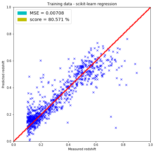
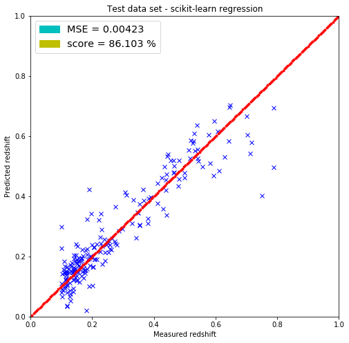
- B, Repeat 2/A using the linear regression class of scikit-learn.
- C, Compare the coefficients of the two implementations.
- D, Use 5 fold cross validation using your linear regression class. Estimate the mean and standard deviation of the MSE of the predictions.
- E, Compare the result of 2/D to the result of KNN regression.
3 Statsmodels
- A Fit linear regression with statsmodels package on the whole dataset. Assess the significance of each color.
- B Iteratvely omit the least significant colors. Compare the $R^2$ of the 5 fits.
- C Validate each 5 combinations of colors using cross validation with 5 folds using your linear regression class. How does the MSE change after omitting the colors? Which is best combination of input colors?
- D, Repeat execise C using a KNN regressor, do you see similar behaviour?
4 Inspection
- A, Select the best combination of input colors found in 3/C, fit the whole dataset, and inspect the residuals of the fit on a residual plot, is there a clear trend?
- B, Inspect the residuals of the fit on a residual plot, identify and color outliers ( where residuals are larger than 3 $ \sigma$ ) .
- C, Identify high levarage data points.
5 Interactions, quadratic terms
- A, Select the best combination of inputs found in 3/C and add interaction between the colors and inspect it’s siginifcance using the whole dataset.
- B, Validate the added interaction using cross validation on 5 folds using your linear regression class or the scikit-learn linear regression class. How does the MSE change after adding interactions?
- C, Add quadratic form of the colors as predictive variables. Asses the significance of the quadratic terms. Which quadratic term is significant?
- D, Create the final model by adding the siginificant quadratic term, interactions and the best input colors. Validate this model using cross validation with 5 folds using your linear regression class. Inspect the final MSE, and compare it to the original model with all colors, the one with the best colors, and the one with interactions. Which is the best?
import numpy as np
import pandas as pd
import matplotlib.pyplot as plt
from matplotlib.patches import Patch
1. Linear regression model based on lecture notes and sources such as Numerical Recipes in C
class LinReg():
    """Linear regression class."""
    def __init__(self):
        """Intialize linear regression."""
        self.coefficients = None

    def fit(self,x_train, y_train):
        """Fit linear regression."""
        A = np.append(x_train, np.ones((x_train.shape[0], 1)), axis=1) # append column for bias
        u, s, vh = np.linalg.svd(A, full_matrices=False, compute_uv=True)
        self.coefficients = np.matmul((np.matmul(u.T, y_train)/s.reshape(s.shape[0],1)).T, vh)[0]
        return self

    def predict(self,x_test):
        """Predict with linear regression."""
        y_test = np.matmul(self.coefficients, (np.append(x_test, np.ones((x_test.shape[0], 1)), axis=1).T))
        y_test = y_test.reshape(y_test.shape[0], 1)
        return y_test
dataset = pd.read_csv("photoz_mini.csv")
print(dataset.columns.values)
colors = ['u', 'g', 'r', 'i', 'z']
['Unnamed: 0' 'id' 'u' 'g' 'r' 'i' 'z' 'redshift']
2. Application
rand_data = np.random.permutation(dataset.values[:,2:8])
# split u, g, r, i, z channels
sets = np.split(rand_data[:,0:5], 5)
test = sets[0]
train = np.concatenate(sets[1:5])
# split redshifts
sets = np.split(rand_data[:,5], 5)
test_redshift = sets[0].reshape(sets[0].shape[0], 1)
train_redshift = np.concatenate(sets[1:5])
train_redshift = train_redshift.reshape(train_redshift.shape[0], 1)
# get shapes
print(train.shape, train_redshift.shape)
print(test.shape, test_redshift.shape)
(800, 5) (800, 1)
(200, 5) (200, 1)
# Linear regression
linreg = LinReg()
reg = linreg.fit(x_train=train, y_train=train_redshift)
print(reg.coefficients)
[-0.0236947 0.05312354 0.25714093 -0.17774562 -0.02446284 -1.39515657]
predicted_redshift = linreg.predict(x_test=test)
# Getting the mean squared error
MSE = np.sum(np.square(predicted_redshift-test_redshift))/test_redshift.shape[0]

# Plotting the results
plt.figure(figsize=(8.,8.))
plt.plot(test_redshift, predicted_redshift, 'bx')
plt.xlim(0,1)
plt.ylim(0,1)
lin = np.linspace(0,1,200)
plt.plot(lin, lin, 'r.')
plt.title('Test data set')
plt.xlabel('Measured redshift')
plt.ylabel('Predicted redshift')
legend_handle = [Patch(facecolor='c', edgecolor='c',
                         label=('MSE = %.5f' % MSE) )]
plt.legend(handles=legend_handle, loc='upper left', fontsize='x-large')
plt.show()
# Same for the training set
predicted_redshift = linreg.predict(x_test=train)
# Getting the mean squared error
MSE = np.sum(np.square(predicted_redshift-train_redshift))/train_redshift.shape[0]

# Plotting the results
plt.figure(figsize=(8.,8.))
plt.plot(train_redshift, predicted_redshift, 'bx')
plt.xlim(0,1)
plt.ylim(0,1)
lin = np.linspace(0,1,200)
plt.plot(lin, lin, 'r.')
plt.title('Training data set')
plt.xlabel('Measured redshift')
plt.ylabel('Predicted redshift')
legend_handle = [Patch(facecolor='c', edgecolor='c',
                         label=('MSE = %.5f' % MSE) )]
plt.legend(handles=legend_handle, loc='upper left', fontsize='x-large')
plt.show()
from sklearn.linear_model import LinearRegression
reg = LinearRegression()
regression = reg.fit(X=train, y=train_redshift)
regression.score(train, train_redshift)
0.805708629407631
print(regression.coef_)
[[-0.0236947 0.05312354 0.25714093 -0.17774562 -0.02446284]]
# skLearn regression
predicted_redshift = reg.predict(X=train).reshape(train.shape[0], 1)
# Getting the mean squared error
MSE = np.sum(np.square(predicted_redshift-train_redshift))/train_redshift.shape[0]

# Plotting the results
plt.figure(figsize=(8.,8.))
plt.plot(train_redshift, predicted_redshift, 'bx')
plt.xlim(0,1)
plt.ylim(0,1)
lin = np.linspace(0,1,200)
plt.plot(lin, lin, 'r.')
plt.title('Training data - scikit-learn regression')
plt.xlabel('Measured redshift')
plt.ylabel('Predicted redshift')
legend_handle = [Patch(facecolor='c', edgecolor='c',
                         label=('MSE = %.5f' % MSE) ),
                 Patch(facecolor='y', edgecolor='y',
                       label=('score = %.3f %%' % (100.*reg.score(train, train_redshift))) )]
plt.legend(handles=legend_handle, loc='upper left', fontsize='x-large')
plt.show()
# Same for the training set
predicted_redshift = reg.predict(X=test)
# Getting the mean squared error
MSE = np.sum(np.square(predicted_redshift-test_redshift))/test_redshift.shape[0]

# Plotting the results
plt.figure(figsize=(8.,8.))
plt.plot(test_redshift, predicted_redshift, 'bx')
plt.xlim(0,1)
plt.ylim(0,1)
lin = np.linspace(0,1,200)
plt.plot(lin, lin, 'r.')
plt.title('Test data set - scikit-learn regression')
plt.xlabel('Measured redshift')
plt.ylabel('Predicted redshift')
legend_handle = [Patch(facecolor='c', edgecolor='c',
                         label=('MSE = %.5f' % MSE) ),
                 Patch(facecolor='y', edgecolor='y',
                       label=('score = %.3f %%' % (100.*reg.score(test, test_redshift))) )]
plt.legend(handles=legend_handle, loc='upper left', fontsize='x-large')
plt.show()
print(linreg.coefficients)
print(reg.coef_[0])
[-0.0236947   0.05312354  0.25714093 -0.17774562 -0.02446284 -1.39515657]
[-0.0236947   0.05312354  0.25714093 -0.17774562 -0.02446284]
The linear regression model included in the scikit-learn package returned the same parameters for the weighs but did not return the bias parameter (-1.32072437) that I have. It most probably has it since the MSEs are the same for both predicting on the test and training set.
from sklearn.model_selection import train_test_split
def k_fold_cross_validation(model, dataset, k=5):
    MSEs = []
    for i in range(k):
        X_train, X_test, y_train, y_test = train_test_split(dataset[colors].values, dataset['redshift'].values,
                                                        test_size=1./k, random_state=i+42, shuffle=True)
        y_train = y_train.reshape(y_train.shape[0], 1)
        y_test = y_test.reshape(y_test.shape[0], 1)
        fit = model.fit(X_train, y_train)
        predicted_redshift = model.predict(X_test).reshape(X_test.shape[0], 1)
        MSEs.append(np.sum(np.square(predicted_redshift-y_test))/y_test.shape[0])
    print("MSE : %.5f +/- %.5f" % (np.mean(MSEs), np.std(MSEs)))
k_fold_cross_validation(LinearRegression(), dataset)
MSE : 0.00789 +/- 0.00110
k_fold_cross_validation(LinReg(), dataset)
MSE : 0.00789 +/- 0.00110
Comparing the regression results to the skLearn KNN algorithm.
from sklearn.neighbors import NearestNeighbors

def sklearn_knn_regression(x2pred, x_train, y_train, k=10):
    neigh = NearestNeighbors(n_neighbors=k)
    neigh.fit(x_train)
    y_pred = []
    for indices in neigh.kneighbors(x2pred, return_distance=False):
        y_pred.append(np.mean(y_train[indices]))
    return np.array(y_pred)

def cross_validate(algo, dataset, splits=5, k=10):
    MSEs = []
    for i in range(splits):
        x_train, x_test, y_train, y_test = train_test_split(dataset[colors].values, dataset['redshift'].values,
                                                        test_size=1./k, random_state=i+42, shuffle=True)
        y_train = y_train.reshape(y_train.shape[0], 1)
        y_test = y_test.reshape(y_test.shape[0], 1)
        y_pred = algo(x_test, x_train, y_train, k)
        y_pred = y_pred.reshape(y_pred.shape[0], 1)
        MSEs.append(np.sum(np.square(y_pred-y_test))/y_test.shape[0])
    print("Mean MSE : %.5f +/- %.5f" % (np.mean(MSEs),np.std(MSEs)))
cross_validate(sklearn_knn_regression, dataset, 5, 17)
Mean MSE : 0.00774 +/- 0.00243
The cross validated value of MSE is approximately the same for KNN and LinearRegression methods of skLearn (and my own). It could mean that the data cannot be fitted linearly or with the k-nearest neighbor method. That is absolutely correct since if it would be possible it would not be researched heavily.
3. Statsmodels
import statsmodels.api as sm
ols_model = sm.OLS(dataset['redshift'].values, dataset[colors].values)
results = ols_model.fit()
print(results.summary(xname=colors))
                            OLS Regression Results
==============================================================================
Dep. Variable:                      y   R-squared:                       0.923
Model:                            OLS   Adj. R-squared:                  0.922
Method:                 Least Squares   F-statistic:                     2369.
Date:                Sun, 07 Oct 2018   Prob (F-statistic):               0.00
Time:                        14:14:26   Log-Likelihood:                 870.12
No. Observations:                1000   AIC:                            -1730.
Df Residuals:                     995   BIC:                            -1706.
Df Model:                           5
Covariance Type:            nonrobust
==============================================================================
                 coef    std err          t      P>|t|      [0.025      0.975]
------------------------------------------------------------------------------
u             -0.1052      0.005    -21.053      0.000      -0.115      -0.095
g              0.1284      0.014      9.454      0.000       0.102       0.155
r              0.3408      0.030     11.432      0.000       0.282       0.399
i             -0.3709      0.034    -10.772      0.000      -0.438      -0.303
z              0.0192      0.023      0.850      0.396      -0.025       0.063
==============================================================================
Omnibus:                      438.904   Durbin-Watson:                   2.028
Prob(Omnibus):                  0.000   Jarque-Bera (JB):             2897.545
Skew:                           1.894   Prob(JB):                         0.00
Kurtosis:                      10.430   Cond. No.                         587.
==============================================================================

Warnings:
[1] Standard Errors assume that the covariance matrix of the errors is correctly specified.
print('Parameters: ', results.params)
print('R2: ', results.rsquared)
print('Significances: ', results.pvalues)
Parameters:  [-0.10523518  0.12835752  0.34079639 -0.37091931  0.01916069]
R2:  0.9225065591482929
Significances:  [1.14349099e-81 2.26884527e-20 1.59402199e-28 1.13785979e-25
 3.95514338e-01]
From the P > |t| significance values above, it can be seen that the parameter z is NOT significant and therefore can be left out of the study since it is greater than the standard 5% significance level.
def significance_check_and_fit(dataset, labels):
    ols_model = sm.OLS(dataset['redshift'].values, dataset[labels].values)
    results = ols_model.fit()
    sign_indices = np.argsort(results.pvalues)
    colors = np.array(labels)
    colors = colors[sign_indices]
    print("R^2 : %.5f" % results.rsquared, "fit for colors: " , colors, "(from most significant to least significant)")
    for k in range(0, colors.size - 1):
        colors = np.resize(colors, colors.size - 1)
        ols_model = sm.OLS(dataset['redshift'].values, dataset[colors].values)
        results = ols_model.fit()
        print("R^2 : %.5f" % results.rsquared, "fit for colors: " , colors )
significance_check_and_fit(dataset, colors)
R^2 : 0.92251 fit for colors:  ['u' 'r' 'i' 'g' 'z'] (from most significant to least significant)
R^2 : 0.92245 fit for colors:  ['u' 'r' 'i' 'g']
R^2 : 0.91549 fit for colors:  ['u' 'r' 'i']
R^2 : 0.83845 fit for colors:  ['u' 'r']
R^2 : 0.76696 fit for colors:  ['u']
The difference in R^2 is not significant after removing the infrared spectrum however it is noticable.
significant_colors = (np.array(colors))[np.argsort(results.pvalues)]
print(significant_colors)
['u' 'r' 'i' 'g' 'z']
def k_fold_cross_validation_with_significance(model, dataset, sign_colors, k=5):
    colors = np.append(sign_colors, -1) # random value to remove first ;)
    MSEs = []
    for arr_cut in range(sign_colors.size):
        colors = np.resize(colors, colors.size - 1)
        print("Fitting for color set : ",       colors)
        print("**************************************")
        for i in range(k):
            X_train, X_test, y_train, y_test = train_test_split(dataset[colors].values, dataset['redshift'].values,
                                                        test_size=1./k, random_state=i+42, shuffle=True)
            y_train = y_train.reshape(y_train.shape[0], 1)
            y_test = y_test.reshape(y_test.shape[0], 1)
            fit = model.fit(X_train, y_train)
            predicted_redshift = model.predict(X_test).reshape(X_test.shape[0], 1)
            MSEs.append(np.sum(np.square(predicted_redshift-y_test))/y_test.shape[0])
        print("MSE : %.5f +/- %.5f\n\n" % (np.mean(MSEs), np.std(MSEs)))
k_fold_cross_validation_with_significance(LinReg(), dataset, significant_colors)
Fitting for color set :  ['u' 'r' 'i' 'g' 'z']
**************************************
MSE : 0.00789 +/- 0.00110


Fitting for color set :  ['u' 'r' 'i' 'g']
**************************************
MSE : 0.00765 +/- 0.00096


Fitting for color set :  ['u' 'r' 'i']
**************************************
MSE : 0.00759 +/- 0.00087


Fitting for color set :  ['u' 'r']
**************************************
MSE : 0.00779 +/- 0.00106


Fitting for color set :  ['u']
**************************************
MSE : 0.00958 +/- 0.00373
I consider the third one the best where the colors are: ‘u’, ‘r’ and ‘i’ and the MSE is the lowest, valued only at (0.00759 +/- 0.00087). It is interesting that the standard deviation is also at its lowest at this combination.
def cross_validate_with_significance(algo, dataset, sign_colors, splits=5, k=10):
    colors = np.append(sign_colors, -1) # random value to remove first ;)
    MSEs = []
    for arr_cut in range(sign_colors.size):
        colors = np.resize(colors, colors.size - 1)
        print("Fitting for color set : ",       colors)
        print("**************************************")
        for i in range(splits):
            x_train, x_test, y_train, y_test = train_test_split(dataset[colors].values, dataset['redshift'].values,
                                                        test_size=1./k, random_state=i+42, shuffle=True)
            y_train = y_train.reshape(y_train.shape[0], 1)
            y_test = y_test.reshape(y_test.shape[0], 1)
            y_pred = algo(x_test, x_train, y_train, k)
            y_pred = y_pred.reshape(y_pred.shape[0], 1)
            MSEs.append(np.sum(np.square(y_pred-y_test))/y_test.shape[0])
        print("Mean MSE : %.5f +/- %.5f\n\n" % (np.mean(MSEs),np.std(MSEs)))
cross_validate_with_significance(sklearn_knn_regression, dataset, significant_colors)
Fitting for color set :  ['u' 'r' 'i' 'g' 'z']
**************************************
Mean MSE : 0.00762 +/- 0.00224


Fitting for color set :  ['u' 'r' 'i' 'g']
**************************************
Mean MSE : 0.00751 +/- 0.00226


Fitting for color set :  ['u' 'r' 'i']
**************************************
Mean MSE : 0.00788 +/- 0.00226


Fitting for color set :  ['u' 'r']
**************************************
Mean MSE : 0.00825 +/- 0.00230


Fitting for color set :  ['u']
**************************************
Mean MSE : 0.00983 +/- 0.00380
It is interesting that here the best fit is for MSE is the color set ‘u’, ‘r’, ‘i’ and ‘g’ valued at (0.00751 +/- 0.00226). However, the result is not that far from the previous one since this one and the other above were the closest now and before as well.
4. Inspection
best_colors_and_redshift = ['u', 'r', 'i', 'redshift'] # based on linear fit

dataset = pd.read_csv("photoz_mini.csv")
data = dataset[best_colors_and_redshift].values
X_train = data[:,0:3]
y_train = data[:,3]

linreg = LinearRegression()
fit = linreg.fit(X_train, y_train)
# Same for the training set
predicted_redshift = linreg.predict(X_train).reshape(X_train.shape[0], 1)

# Getting the mean squared error
MSE = np.sum(np.square(predicted_redshift-y_train.reshape(y_train.shape[0], 1)))/y_train.shape[0]

# Plotting the results
plt.figure(figsize=(8.,8.))
plt.scatter(y_train, predicted_redshift, c='b', marker='x')
plt.xlim(0,1)
plt.ylim(0,1)
lin = np.linspace(0,1,300)
plt.scatter(lin, lin, c='r', marker='.')
plt.title('Whole dataset - scikit-learn regression for colors: u, r, i')
plt.xlabel('Measured redshift')
plt.ylabel('Predicted redshift')
legend_handle = [Patch(facecolor='c', edgecolor='c',
                         label=('MSE = %.5f' % MSE))]
plt.legend(handles=legend_handle, loc='upper left', fontsize='x-large')
plt.show()
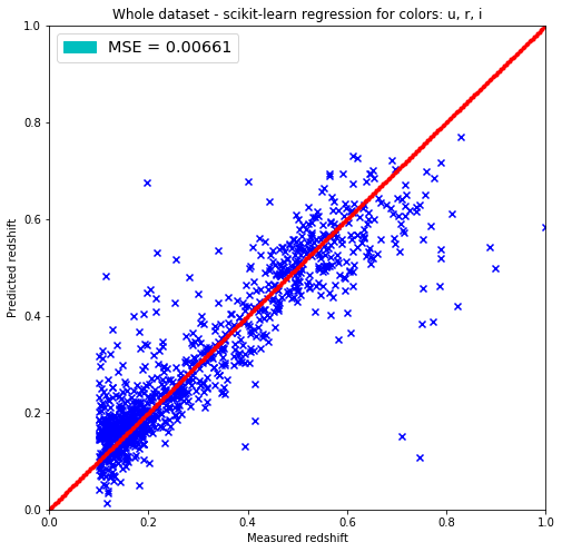
It seems that the fit does not work very well under redshift 0.1. There’s a waveing of the data and huge outliers as well. It seems that there are 2 clusters as well around 0.15 and at 0.55 and the data is more rare around 0.4.
errs = np.abs(predicted_redshift-y_train.reshape(y_train.shape[0], 1))/y_train.shape[0]
sigma = np.std(errs)
print(errs.shape)
(1000, 1)
non_outliers = []
outliers = []
for ind in range(0, errs.size):
    if errs[ind] < 3*sigma:
        non_outliers.append(ind)
    else:
        outliers.append(ind)
# Same for the training set
predicted_redshift = linreg.predict(X_train).reshape(X_train.shape[0], 1)
# Plotting the results
plt.figure(figsize=(8.,8.))
# Removing outliers from both predicted_redshift, and y_train sets
predicted_redshift_og = predicted_redshift
predicted_redshift = predicted_redshift_og[non_outliers]
outlier_redshift = predicted_redshift_og[outliers]
# Same for measured redshifts
y_train_og = y_train.reshape(y_train.shape[0], 1)
y_train = y_train_og[non_outliers]
outlier_y = y_train_og[outliers]
# Getting the mean squared error
MSE = np.sum(np.square(predicted_redshift-y_train))/y_train.shape[0]
plt.scatter(y_train, predicted_redshift, c='b', marker='x')
plt.scatter(outlier_y, outlier_redshift, c='r', marker='o')
plt.xlim(0,1)
plt.ylim(0,1)
lin = np.linspace(0,1,300)
plt.scatter(lin, lin, c='r', marker='.')
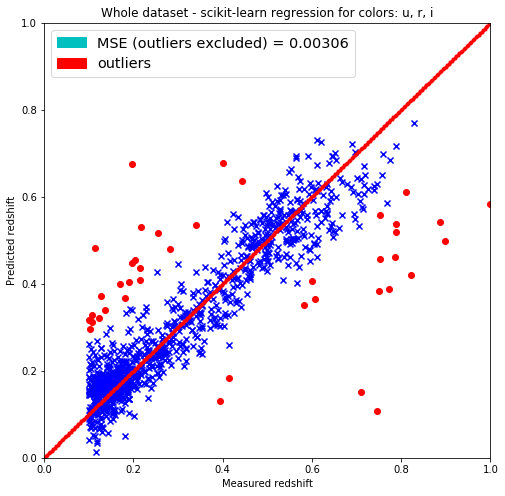
plt.title('Whole dataset - scikit-learn regression for colors: u, r, i')
plt.xlabel('Measured redshift')
plt.ylabel('Predicted redshift')
legend_handle = [Patch(facecolor='c', edgecolor='c',
label=('MSE (outliers excluded) = %.5f' % MSE)),
Patch(facecolor='r', edgecolor='r',
label=('outliers'))]
plt.legend(handles=legend_handle, loc='upper left', fontsize='x-large')
plt.show()
# Best colors fit with OLS
y_train = dataset[best_colors_and_redshift].values[:,3]
X_train = dataset[best_colors_and_redshift].values[:,0:3]
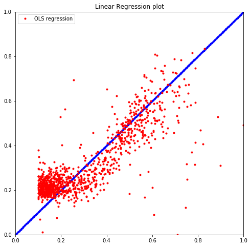
lm = sm.OLS(y_train, X_train).fit()
print("The R^2 value is %.5f" % lm.rsquared)
plt.figure(figsize=(8.,8.))
plt.xlim(0,1)
plt.ylim(0,1)
lin = np.linspace(0,1,300)
plt.scatter(lin, lin, c='b', marker='.')
plt.plot(y_train, lm.predict(), 'r.', label="OLS regression")
plt.title("Linear Regression plot")
plt.legend()
The R^2 value is 0.91549


<matplotlib.legend.Legend at 0x7fb12e7cbc88>
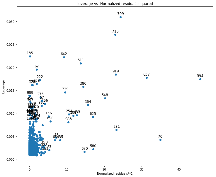
from statsmodels.graphics.regressionplots import plot_leverage_resid2
fig, ax = plt.subplots(figsize=(12,10))
fig = plot_leverage_resid2(lm, ax=ax)
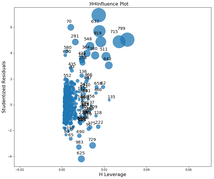
fig, ax = plt.subplots(figsize=(12,10))
fig = sm.graphics.influence_plot(lm, ax=ax)
5. Interactions, quadratic terms
import statsmodels.formula.api as smf
# Calculating length like quantity
mod = smf.ols(formula="redshift ~ np.sqrt(u**2+r**2+i**2)", data=dataset)
results = mod.fit()
print(results.summary())
                            OLS Regression Results
==============================================================================
Dep. Variable:               redshift   R-squared:                       0.722
Model:                            OLS   Adj. R-squared:                  0.721
Method:                 Least Squares   F-statistic:                     2586.
Date:                Sun, 07 Oct 2018   Prob (F-statistic):          2.50e-279
Time:                        14:14:31   Log-Likelihood:                 888.76
No. Observations:                1000   AIC:                            -1774.
Df Residuals:                     998   BIC:                            -1764.
Df Model:                           1
Covariance Type:            nonrobust
=====================================================================================================
                                        coef    std err          t      P>|t|      [0.025      0.975]
-----------------------------------------------------------------------------------------------------
Intercept                            -2.2154      0.050    -44.496      0.000      -2.313      -2.118
np.sqrt(u ** 2 + r ** 2 + i ** 2)     0.0753      0.001     50.855      0.000       0.072       0.078
==============================================================================
Omnibus:                      122.604   Durbin-Watson:                   2.005
Prob(Omnibus):                  0.000   Jarque-Bera (JB):             1164.541
Skew:                           0.016   Prob(JB):                    1.33e-253
Kurtosis:                       8.287   Cond. No.                         532.
==============================================================================

Warnings:
[1] Standard Errors assume that the covariance matrix of the errors is correctly specified.
# Fitting for all parameters
mod = smf.ols(formula="redshift ~ u+r+i", data=dataset)
results = mod.fit()
print(results.summary())
                            OLS Regression Results
==============================================================================
Dep. Variable:               redshift   R-squared:                       0.814
Model:                            OLS   Adj. R-squared:                  0.813
Method:                 Least Squares   F-statistic:                     1453.
Date:                Sun, 07 Oct 2018   Prob (F-statistic):               0.00
Time:                        14:14:31   Log-Likelihood:                 1090.6
No. Observations:                1000   AIC:                            -2173.
Df Residuals:                     996   BIC:                            -2154.
Df Model:                           3
Covariance Type:            nonrobust
==============================================================================
                 coef    std err          t      P>|t|      [0.025      0.975]
------------------------------------------------------------------------------
Intercept     -1.4395      0.055    -26.314      0.000      -1.547      -1.332
u             -0.0037      0.004     -0.974      0.330      -0.011       0.004
r              0.3647      0.015     24.655      0.000       0.336       0.394
i             -0.2755      0.015    -17.967      0.000      -0.306      -0.245
==============================================================================
Omnibus:                      323.702   Durbin-Watson:                   1.989
Prob(Omnibus):                  0.000   Jarque-Bera (JB):             5026.464
Skew:                           1.048   Prob(JB):                         0.00
Kurtosis:                      13.782   Cond. No.                         733.
==============================================================================

Warnings:
[1] Standard Errors assume that the covariance matrix of the errors is correctly specified.
# Adding interaction to best parameters
mod = smf.ols(formula="redshift ~ u*r*i", data=dataset)
results = mod.fit()
print(results.summary())
                            OLS Regression Results
==============================================================================
Dep. Variable:               redshift   R-squared:                       0.830
Model:                            OLS   Adj. R-squared:                  0.829
Method:                 Least Squares   F-statistic:                     692.1
Date:                Sun, 07 Oct 2018   Prob (F-statistic):               0.00
Time:                        14:33:16   Log-Likelihood:                 1135.6
No. Observations:                1000   AIC:                            -2255.
Df Residuals:                     992   BIC:                            -2216.
Df Model:                           7
Covariance Type:            nonrobust
==============================================================================
                 coef    std err          t      P>|t|      [0.025      0.975]
------------------------------------------------------------------------------
Intercept     75.5142      9.873      7.649      0.000      56.140      94.888
u             -3.3060      0.452     -7.317      0.000      -4.193      -2.419
r             -4.4199      0.728     -6.074      0.000      -5.848      -2.992
u:r            0.2072      0.032      6.382      0.000       0.143       0.271
i             -4.3049      0.613     -7.027      0.000      -5.507      -3.103
u:i            0.1725      0.029      6.018      0.000       0.116       0.229
r:i            0.2515      0.031      8.059      0.000       0.190       0.313
u:r:i         -0.0109      0.001     -7.709      0.000      -0.014      -0.008
==============================================================================
Omnibus:                      298.041   Durbin-Watson:                   1.961
Prob(Omnibus):                  0.000   Jarque-Bera (JB):             6500.267
Skew:                           0.822   Prob(JB):                         0.00
Kurtosis:                      15.381   Cond. No.                     2.97e+07
==============================================================================

Warnings:
[1] Standard Errors assume that the covariance matrix of the errors is correctly specified.
[2] The condition number is large, 2.97e+07. This might indicate that there are
strong multicollinearity or other numerical problems.
dataset = dataset.assign(ur=dataset['u']*dataset['r'])
dataset = dataset.assign(ri=dataset['r']*dataset['i'])
dataset = dataset.assign(ui=dataset['u']*dataset['i'])
dataset = dataset.assign(uri=dataset['u']*dataset['r']*dataset['i'])
print(results.pvalues.sort_values())
r:i          2.204473e-15
u:r:i        3.071793e-14
Intercept    4.787405e-14
u            5.236449e-13
i            3.911423e-12
u:r          2.686197e-10
r            1.779040e-09
u:i          2.476056e-09
dtype: float64
significant_colors = np.array(['ri', 'uri', 'u', 'i', 'ur', 'r', 'ui'])
k_fold_cross_validation_with_significance(LinearRegression(), dataset, significant_colors)
Fitting for color set :  ['ri' 'uri' 'u' 'i' 'ur' 'r' 'ui']
**************************************
MSE : 0.00715 +/- 0.00082


Fitting for color set :  ['ri' 'uri' 'u' 'i' 'ur' 'r']
**************************************
MSE : 0.00710 +/- 0.00072


Fitting for color set :  ['ri' 'uri' 'u' 'i' 'ur']
**************************************
MSE : 0.00709 +/- 0.00070


Fitting for color set :  ['ri' 'uri' 'u' 'i']
**************************************
MSE : 0.00702 +/- 0.00074


Fitting for color set :  ['ri' 'uri' 'u']
**************************************
MSE : 0.00737 +/- 0.00112


Fitting for color set :  ['ri' 'uri']
**************************************
MSE : 0.00763 +/- 0.00129


Fitting for color set :  ['ri']
**************************************
MSE : 0.00788 +/- 0.00143
k_fold_cross_validation_with_significance(LinReg(), dataset, significant_colors)
Fitting for color set :  ['ri' 'uri' 'u' 'i' 'ur' 'r' 'ui']
**************************************
MSE : 0.00715 +/- 0.00082


Fitting for color set :  ['ri' 'uri' 'u' 'i' 'ur' 'r']
**************************************
MSE : 0.00710 +/- 0.00072


Fitting for color set :  ['ri' 'uri' 'u' 'i' 'ur']
**************************************
MSE : 0.00709 +/- 0.00070


Fitting for color set :  ['ri' 'uri' 'u' 'i']
**************************************
MSE : 0.00702 +/- 0.00074


Fitting for color set :  ['ri' 'uri' 'u']
**************************************
MSE : 0.00737 +/- 0.00112


Fitting for color set :  ['ri' 'uri']
**************************************
MSE : 0.00763 +/- 0.00129


Fitting for color set :  ['ri']
**************************************
MSE : 0.00788 +/- 0.00143
The best combination of colors and interactions seems to be the combination: ri, uri, u, i, ur.
# Adding interaction to best parameters
mod = smf.ols(formula="redshift ~ np.square(u)+np.square(r)+np.square(i)+u*r*i", data=dataset)
results = mod.fit()
print(results.summary())
                            OLS Regression Results
==============================================================================
Dep. Variable:               redshift   R-squared:                       0.826
Model:                            OLS   Adj. R-squared:                  0.825
Method:                 Least Squares   F-statistic:                     523.7
Date:                Sun, 07 Oct 2018   Prob (F-statistic):               0.00
Time:                        14:39:41   Log-Likelihood:                 1125.0
No. Observations:                1000   AIC:                            -2230.
Df Residuals:                     990   BIC:                            -2181.
Df Model:                           9
Covariance Type:            nonrobust
================================================================================
                   coef    std err          t      P>|t|      [0.025      0.975]
--------------------------------------------------------------------------------
Intercept        1.3576      1.040      1.305      0.192      -0.684       3.399
np.square(u)     0.0153      0.004      3.770      0.000       0.007       0.023
np.square(r)     0.0292      0.041      0.710      0.478      -0.051       0.110
np.square(i)     0.0878      0.036      2.428      0.015       0.017       0.159
u               -0.1749      0.110     -1.595      0.111      -0.390       0.040
r                1.1304      0.403      2.804      0.005       0.339       1.921
u:r              0.0006      0.025      0.024      0.981      -0.049       0.051
i               -1.1630      0.396     -2.938      0.003      -1.940      -0.386
u:i             -0.0271      0.026     -1.038      0.299      -0.078       0.024
r:i             -0.0979      0.076     -1.295      0.196      -0.246       0.050
==============================================================================
Omnibus:                      295.957   Durbin-Watson:                   2.009
Prob(Omnibus):                  0.000   Jarque-Bera (JB):            10206.776
Skew:                           0.661   Prob(JB):                         0.00
Kurtosis:                      18.595   Cond. No.                     3.99e+05
==============================================================================

Warnings:
[1] Standard Errors assume that the covariance matrix of the errors is correctly specified.
[2] The condition number is large, 3.99e+05. This might indicate that there are
strong multicollinearity or other numerical problems.
The most significant squares seem to be i, u and r in this order, but I am going to fit and cross validate for all and by significance ordering with OLS and cross-validate with KNN.
dataset = dataset.assign(uu=dataset['u']*dataset['u'])
dataset = dataset.assign(ii=dataset['i']*dataset['i'])
dataset = dataset.assign(rr=dataset['r']*dataset['r'])
print(results.pvalues.sort_values())
np.square(u)    0.000173
i               0.003380
r               0.005144
np.square(i)    0.015362
u               0.110974
Intercept       0.192202
r:i             0.195508
u:i             0.299343
np.square(r)    0.477669
u:r             0.980820
dtype: float64
significant_colors = np.array(['i', 'u', 'uri', 'ur', 'r', 'ui', 'ii', 'uu', 'ri', 'rr'])
k_fold_cross_validation_with_significance(LinearRegression(), dataset, significant_colors)
Fitting for color set :  ['i' 'u' 'uri' 'ur' 'r' 'ui' 'ii' 'uu' 'ri' 'rr']
**************************************
MSE : 0.00699 +/- 0.00100


Fitting for color set :  ['i' 'u' 'uri' 'ur' 'r' 'ui' 'ii' 'uu' 'ri']
**************************************
MSE : 0.00697 +/- 0.00099


Fitting for color set :  ['i' 'u' 'uri' 'ur' 'r' 'ui' 'ii' 'uu']
**************************************
MSE : 0.00689 +/- 0.00101


Fitting for color set :  ['i' 'u' 'uri' 'ur' 'r' 'ui' 'ii']
**************************************
MSE : 0.00686 +/- 0.00102


Fitting for color set :  ['i' 'u' 'uri' 'ur' 'r' 'ui']
**************************************
MSE : 0.00692 +/- 0.00097


Fitting for color set :  ['i' 'u' 'uri' 'ur' 'r']
**************************************
MSE : 0.00695 +/- 0.00093


Fitting for color set :  ['i' 'u' 'uri' 'ur']
**************************************
MSE : 0.00703 +/- 0.00092


Fitting for color set :  ['i' 'u' 'uri']
**************************************
MSE : 0.00707 +/- 0.00098


Fitting for color set :  ['i' 'u']
**************************************
MSE : 0.00741 +/- 0.00139


Fitting for color set :  ['i']
**************************************
MSE : 0.00774 +/- 0.00170
The best combination of all: i, u, uri, ur, r, ui, ii.
Compared to the all previous models this seems to be the best. If I did the outlier dropping and k-fold cross validation for the KNN I suppose the KNN model would be the best of all.
@Regards, Alex

Alex Olar
Christian, foodie, physicist, tech enthusiast