
Logistic regression and SVM classification on famous Titanic data from Kaggle
- 22 minsimport numpy as np
import pandas as pd
import matplotlib.pyplot as plt
import seaborn as sns
Data
I acquired data from Kaggle. This is collected from the passengers on the famous Titanic ship. Analyzing the data there are some pretty interesting results.
train = pd.read_csv("train.csv")
train.head(n=10)
| Survived | Pclass | Name | Sex | Age | |
|---|---|---|---|---|---|
| 1 | 0 | 3 | Braund, Mr. Owen Harris | male | 22.0 |
| 2 | 1 | 1 | Cumings, Mrs. John Bradley (Florence Briggs Th... | female | 38.0 |
| 3 | 1 | 3 | Heikkinen, Miss. Laina | female | 26.0 |
| 4 | 1 | 1 | Futrelle, Mrs. Jacques Heath (Lily May Peel) | female | 35.0 |
// data is left out on purpose for better visualization
sns.heatmap(train.isna(), cbar=False), train.info()
<class 'pandas.core.frame.DataFrame'>
RangeIndex: 891 entries, 0 to 890
Data columns (total 12 columns):
PassengerId    891 non-null int64
Survived       891 non-null int64
Pclass         891 non-null int64
Name           891 non-null object
Sex            891 non-null object
Age            714 non-null float64
SibSp          891 non-null int64
Parch          891 non-null int64
Ticket         891 non-null object
Fare           891 non-null float64
Cabin          204 non-null object
Embarked       889 non-null object
dtypes: float64(2), int64(5), object(5)
memory usage: 83.6+ KB


(<matplotlib.axes._subplots.AxesSubplot at 0x7fbff8af45c0>, None)
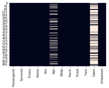
Cabin number and age is not present for everyone, I set the cabin number to unknown instead of NaN and where age was missing I set it to the mean of the dataset.
# Fill age with mean because only some are missing
train['Age'] = train['Age'].fillna(train['Age'].dropna().mean())
# Set NaN for Cabin to Unknown because if it would be dropped we would loose ~70% of data
train['Cabin'] = train['Cabin'].fillna('Unknown')
# For any other let's drop the record
train = train.dropna()
sns.heatmap(train.isna(), cbar=False), train.info()
<class 'pandas.core.frame.DataFrame'>
Int64Index: 889 entries, 0 to 890
Data columns (total 12 columns):
PassengerId    889 non-null int64
Survived       889 non-null int64
Pclass         889 non-null int64
Name           889 non-null object
Sex            889 non-null object
Age            889 non-null float64
SibSp          889 non-null int64
Parch          889 non-null int64
Ticket         889 non-null object
Fare           889 non-null float64
Cabin          889 non-null object
Embarked       889 non-null object
dtypes: float64(2), int64(5), object(5)
memory usage: 90.3+ KB


(<matplotlib.axes._subplots.AxesSubplot at 0x7fbff47e7198>, None)
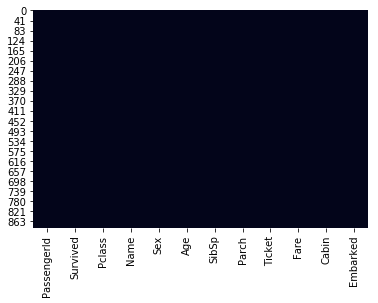
Where there were still missing data I dropped those that contained NaN.
fig = plt.figure(figsize=(7, 6))
sns.set(style="ticks")
sns.boxplot(x="Pclass", y="Age", data=train,
            whis="range", palette="vlag")
plt.title("Age - Class, mean and standard deviation")
plt.show()
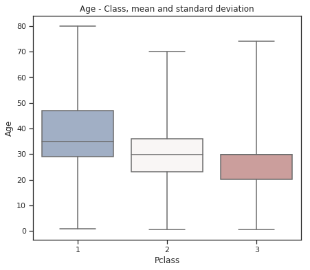
Older people buy first class tickets mostly.
fig = plt.figure(figsize=(7, 6))
sns.set(style="ticks")
sns.boxplot(x="Sex", y="Pclass", data=train,
            whis="range", palette="winter")
plt.title("Gender - Class, mean and standard deviation")
plt.show()
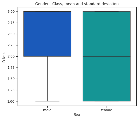
Males buy less first class tickets.
fig = plt.figure(figsize=(7, 6))
sns.set(style="ticks")
sns.boxplot(x="Sex", y="Age", data=train,
            whis="range", palette="vlag")
plt.title("Age - Gender, mean and standard deviation")
plt.show()
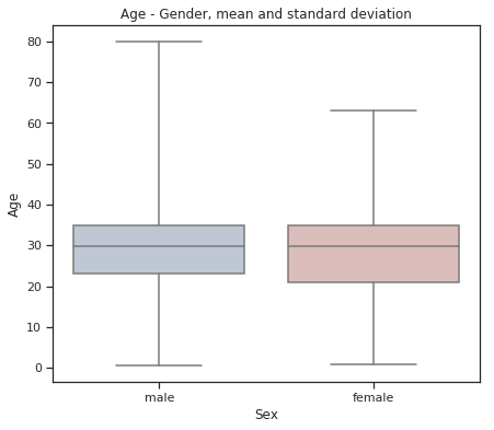
fig = plt.figure(figsize=(7, 6))
sns.set(style="ticks")
sns.boxplot(x="Survived", y="Age", data=train,
            whis="range", palette="vlag")
plt.title("Age - Survived, mean and standard deviation")
plt.show()
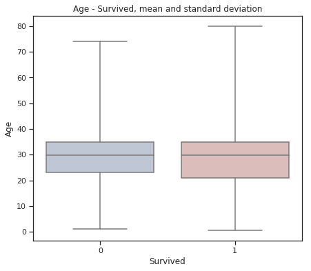
fig = plt.figure(figsize=(7, 6))
sns.set(style="ticks")
sns.boxplot(x="Sex", y="Fare", data=train,
            whis="range", palette="vlag")
plt.title("Fare - Sex, mean and standard deviation")
plt.show()
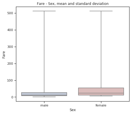
Females bought more expensive tickets.
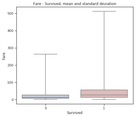
# JK but the fare for survival was higher. :DDDD
fig = plt.figure(figsize=(7, 6))
sns.set(style="ticks")
sns.boxplot(x="Survived", y="Fare", data=train,
            whis="range", palette="vlag")
plt.title("Fare - Survived, mean and standard deviation")
plt.show()
embarked = set(train['Embarked'].values)
embarked = dict(zip(embarked, range(len(embarked))))
embarked
{'C': 0, 'Q': 1, 'S': 2}
train['Embarked'] = train['Embarked'].map(lambda value: embarked[value])
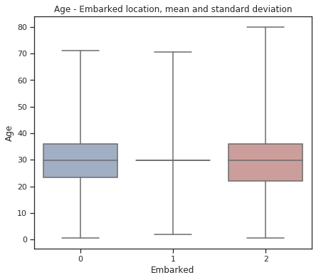
fig = plt.figure(figsize=(7, 6))
sns.set(style="ticks")
sns.boxplot(x="Embarked", y="Age", data=train,
            whis="range", palette="vlag")
plt.title("Age - Embarked location, mean and standard deviation")
plt.show()
gender = set(train['Sex'].values)
gender = dict(zip(gender, range(len(gender))))
gender
{'female': 0, 'male': 1}
train['Sex'] = train['Sex'].map(lambda value: gender[value])
numerical_data = train[['Pclass', 'Sex', 'Age', 'SibSp', 'Parch', 'Fare', 'Embarked']]
survived = train['Survived']
from sklearn.preprocessing import normalize
numerical_data = normalize(numerical_data)
fig = plt.figure(figsize=(7, 6)) sns.set(style=”ticks”) sns.boxplot(x=”Embarked”, y=”Fare”, data=train, whis=”range”, palette=”vlag”) plt.title(“Gender - Class, mean and standard deviation”) plt.show()
Logistic regression
from sklearn.model_selection import train_test_split
from sklearn.linear_model import LogisticRegression
X_train, X_test, y_train, y_test = train_test_split(numerical_data, survived, test_size=0.2,
random_state=42, shuffle=True)
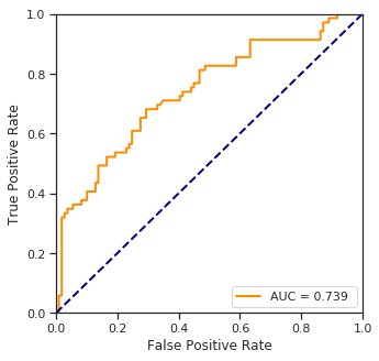
clf = LogisticRegression().fit(X_train, y_train)
y_pred = clf.predict(X_test)
y_proba = clf.decision_function(X_test)
from sklearn.metrics import accuracy_score, auc, roc_curve, classification_report
print("Accuracy score: %.2f%%" % (100.*accuracy_score(y_test, y_pred)))
Accuracy score: 70.79%
fpr, tpr, threshold = roc_curve(y_test, y_proba)

plt.figure(figsize=(5.,5.))
lw = 2
plt.plot(fpr, tpr, color='darkorange',lw=lw, label="AUC = %.3f " % auc(fpr, tpr))
plt.plot([0, 1], [0, 1], color='navy', lw=lw, linestyle='--')
plt.xlim([0.0, 1.0])
plt.ylim([0.0, 1.0])
plt.xlabel('False Positive Rate')
plt.ylabel('True Positive Rate')
plt.legend(loc="lower right")
plt.show()
from matplotlib import colors as mpl_colors
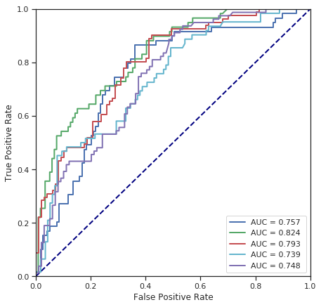
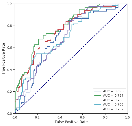
def cross_validate(model, data, labels, k_fold=5, shuffle=True):
plt.figure(figsize=(7.,7.))
lw = 2
colors = list(mpl_colors.BASE_COLORS.keys())
plt.plot([0, 1], [0, 1], color='navy', lw=lw, linestyle='--')
for i in range(k_fold):
X_train, X_test, y_train, y_test = train_test_split(numerical_data, survived, test_size=0.2,
random_state=42*i+k_fold, shuffle=shuffle)
clf = model.fit(X_train, y_train)
y_pred = clf.predict(X_test)
y_proba = clf.decision_function(X_test)
print("Fold %d - accuracy score: %.2f%%" % ((i+1), 100.*accuracy_score(y_test, y_pred)))
fpr, tpr, threshold = roc_curve(y_test, y_proba)
plt.plot(fpr, tpr, color=colors[i], lw=lw, label="AUC = %.3f " % auc(fpr, tpr))
plt.xlim([0.0, 1.0])
plt.ylim([0.0, 1.0])
plt.xlabel('False Positive Rate')
plt.ylabel('True Positive Rate')
plt.legend(loc="lower right")
plt.show()
print("*******************************************************")
print("Classification report for the last fold:")
print(classification_report(y_test, y_pred, target_names=['not survived', 'survived']))
print("*******************************************************\n\n\n")
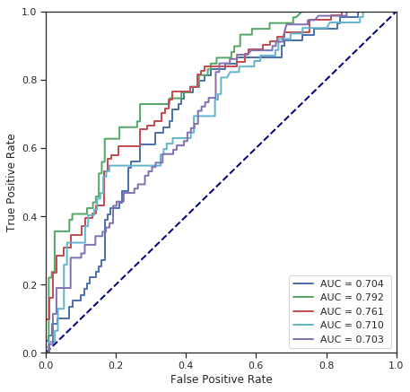
cross_validate(LogisticRegression(), numerical_data, survived) # with shuffle
Fold 1 - accuracy score: 68.54%
Fold 2 - accuracy score: 74.72%
Fold 3 - accuracy score: 68.54%
Fold 4 - accuracy score: 71.91%
Fold 5 - accuracy score: 63.48%
*******************************************************
Classification report for the last fold:
              precision    recall  f1-score   support

not survived       0.63      0.81      0.71        99
    survived       0.63      0.42      0.50        79

 avg / total       0.63      0.63      0.62       178

*******************************************************
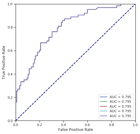
cross_validate(LogisticRegression(), numerical_data, survived, shuffle=False) # without shuffle
Fold 1 - accuracy score: 72.47%
Fold 2 - accuracy score: 72.47%
Fold 3 - accuracy score: 72.47%
Fold 4 - accuracy score: 72.47%
Fold 5 - accuracy score: 72.47%
*******************************************************
Classification report for the last fold:
              precision    recall  f1-score   support

not survived       0.76      0.84      0.80       115
    survived       0.64      0.51      0.57        63

 avg / total       0.72      0.72      0.72       178

*******************************************************
SVM
I used different SVM classifiers with different kernels to estimate the survivals.
from sklearn.svm import LinearSVC, SVC, NuSVC
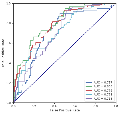
cross_validate(LinearSVC(C=1), numerical_data, survived)
Fold 1 - accuracy score: 68.54%
Fold 2 - accuracy score: 76.97%
Fold 3 - accuracy score: 69.10%
Fold 4 - accuracy score: 70.79%
Fold 5 - accuracy score: 65.73%
*******************************************************
Classification report for the last fold:
              precision    recall  f1-score   support

not survived       0.65      0.84      0.73        99
    survived       0.68      0.43      0.53        79

 avg / total       0.66      0.66      0.64       178

*******************************************************
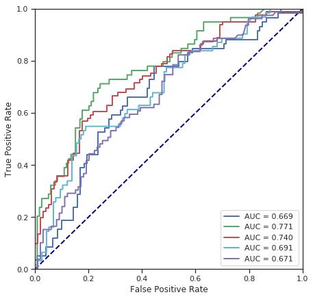
cross_validate(SVC(kernel='linear', C=1), numerical_data, survived)
Fold 1 - accuracy score: 65.17%
Fold 2 - accuracy score: 73.03%
Fold 3 - accuracy score: 65.73%
Fold 4 - accuracy score: 71.35%
Fold 5 - accuracy score: 61.80%
*******************************************************
Classification report for the last fold:
              precision    recall  f1-score   support

not survived       0.62      0.81      0.70        99
    survived       0.61      0.38      0.47        79

 avg / total       0.62      0.62      0.60       178

*******************************************************
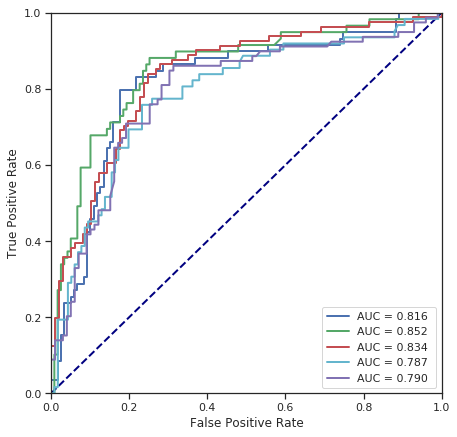
cross_validate(NuSVC(), numerical_data, survived)
Fold 1 - accuracy score: 80.34%
Fold 2 - accuracy score: 78.65%
Fold 3 - accuracy score: 75.28%
Fold 4 - accuracy score: 73.03%
Fold 5 - accuracy score: 75.84%
*******************************************************
Classification report for the last fold:
              precision    recall  f1-score   support

not survived       0.77      0.80      0.79        99
    survived       0.74      0.71      0.72        79

 avg / total       0.76      0.76      0.76       178

*******************************************************
cross_validate(SVC(kernel='poly', degree=3), numerical_data, survived)
Fold 1 - accuracy score: 66.85%
Fold 2 - accuracy score: 66.85%
Fold 3 - accuracy score: 54.49%
Fold 4 - accuracy score: 65.17%
Fold 5 - accuracy score: 55.62%
*******************************************************
Classification report for the last fold:
              precision    recall  f1-score   support

not survived       0.56      1.00      0.71        99
    survived       0.00      0.00      0.00        79

 avg / total       0.31      0.56      0.40       178

*******************************************************


/opt/conda/lib/python3.6/site-packages/sklearn/metrics/classification.py:1135: UndefinedMetricWarning: Precision and F-score are ill-defined and being set to 0.0 in labels with no predicted samples.
  'precision', 'predicted', average, warn_for)
cross_validate(SVC(C=1), numerical_data, survived) # radial kernel by default
Fold 1 - accuracy score: 65.73%
Fold 2 - accuracy score: 74.16%
Fold 3 - accuracy score: 65.73%
Fold 4 - accuracy score: 71.35%
Fold 5 - accuracy score: 61.80%
*******************************************************
Classification report for the last fold:
              precision    recall  f1-score   support

not survived       0.62      0.81      0.70        99
    survived       0.61      0.38      0.47        79

 avg / total       0.62      0.62      0.60       178

*******************************************************
Most important features
from sklearn.feature_selection import RFECV

X_train, X_test, y_train, y_test = train_test_split(
    numerical_data, survived, test_size=0.2,
    random_state=42, shuffle=True)
svc = SVC(kernel="linear")
# The "accuracy" scoring is proportional to the number of correct
# classifications
rfecv = RFECV(estimator=svc, step=1, cv=5,
              scoring='accuracy')
rfecv.fit(X_train, y_train)

print("Optimal number of features : %d" % rfecv.n_features_)

# Plot number of features VS. cross-validation scores
plt.figure()
plt.xlabel("Number of features selected")
plt.ylabel("Cross validation score (nb of correct classifications)")
plt.plot(range(1, len(rfecv.grid_scores_) + 1), rfecv.grid_scores_)
plt.show()
Optimal number of features : 4
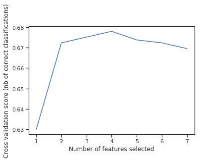
It means that the last feature, namely where people embarked the ship does not matter at all and only lowers accuracy.
Validation
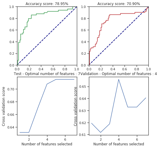
def svm_behaviour_check(data, labels, C=1.0, cache_size=200, class_weight=None, coef0=0.0,
    decision_function_shape='ovr', degree=3, gamma='auto',
    max_iter=-1, probability=False, random_state=None, shrinking=True,
    tol=0.001, verbose=False):

    dat = data[:, 0:4]

    X_train, X_test, y_train, y_test = train_test_split(data, labels, test_size=0.3,
        random_state=42, shuffle=True)
    X_test, X_valid, y_test, y_valid = train_test_split(X_test, y_test, test_size=0.5,
        random_state=137, shuffle=True)

    clf = SVC(C=C, cache_size=cache_size, class_weight=class_weight, coef0=coef0,
    decision_function_shape=decision_function_shape, degree=degree, gamma=gamma, kernel="linear",
    max_iter=max_iter, probability=probability, random_state=random_state, shrinking=shrinking,
    tol=tol, verbose=verbose).fit(X_train, y_train)

    test_pred = clf.predict(X_test)
    valid_pred = clf.predict(X_valid)
    test_proba = clf.decision_function(X_test)
    valid_proba = clf.decision_function(X_valid)

    plt.figure(figsize=(8, 8))
    plt.subplot(221)
    plt.xlim(0,1)
    plt.ylim(0,1)
    plt.plot([0, 1], [0, 1], color='navy', lw=lw, linestyle='--')
    plt.title("Accuracy score: %.2f%%" % (100.*accuracy_score(y_test, test_pred)))
    fpr, tpr, threshold = roc_curve(y_test, test_proba)
    plt.plot(fpr, tpr, color='g', lw=lw, label="AUC = %.3f " % auc(fpr, tpr))
    plt.subplot(222)
    plt.xlim(0,1)
    plt.ylim(0,1)
    plt.plot([0, 1], [0, 1], color='navy', lw=lw, linestyle='--')
    plt.title("Accuracy score: %.2f%%" % (100.*accuracy_score(y_valid, valid_pred)))
    fpr, tpr, threshold = roc_curve(y_valid, valid_proba)
    plt.plot(fpr, tpr, color='r', lw=lw, label="AUC = %.3f " % auc(fpr, tpr))

    rfecv = RFECV(estimator=clf, step=1, cv=5,
              scoring='accuracy')
    rfecv.fit(X_test, y_test)

    # Plot number of features VS. cross-validation scores
    plt.subplot(223)
    plt.title("Test - Optimal number of features : %d" % rfecv.n_features_)
    plt.xlabel("Number of features selected")
    plt.ylabel("Cross validation score")
    plt.plot(range(1, len(rfecv.grid_scores_) + 1), rfecv.grid_scores_)

    rfecv = RFECV(estimator=clf, step=1, cv=5,
              scoring='accuracy')
    rfecv.fit(X_valid, y_valid)

    # Plot number of features VS. cross-validation scores
    plt.subplot(224)
    plt.title("Validation - Optimal number of features : %d" % rfecv.n_features_)
    plt.xlabel("Number of features selected")
    plt.ylabel("Cross validation score")
    plt.plot(range(1, len(rfecv.grid_scores_) + 1), rfecv.grid_scores_)

    plt.show()
svm_behaviour_check(numerical_data, survived, C=25.6, gamma=1.6, shrinking=False, coef0=42)
svm_behaviour_check(numerical_data, survived, C=25.6, gamma=1.6, shrinking=False, coef0=1378)

svm_behaviour_check(numerical_data, survived, C=61166.6, gamma=1.6, shrinking=False, coef0=42)
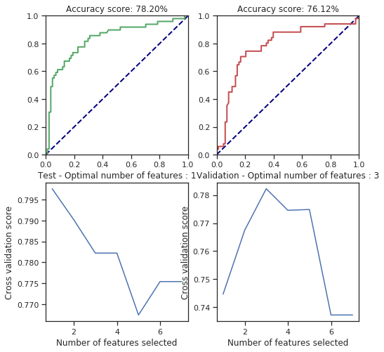
svm_behaviour_check(numerical_data, survived, C=25.6, gamma=1379, shrinking=False, coef0=42)

svm_behaviour_check(numerical_data, survived, C=25.6, gamma=1.6, shrinking=True, coef0=42)

For some parameters there is considerable change but most of them are fitted correctly. However, I only tried few of the parameters so I can’t say more of this. However, the cross validated feature selection scores are pretty bad regarding the results.

Alex Olar
Christian, foodie, physicist, tech enthusiast