
Image classification using machine learning on MNIST dataset
- 16 minsVery basic image classification using machine learning techniques
import mnist
import skimage
import numpy as np
import matplotlib.pyplot as plt
import itertools
from sklearn.model_selection import train_test_split as tts
from sklearn.neighbors import KNeighborsClassifier
from sklearn.linear_model import LogisticRegression
from sklearn.metrics import confusion_matrix
Acquiring the dataset
Using the mnist package I am acquiring the dataset from the MNIST library. The package is capable of returning a training and a test set as well. First of all, I am going to test out my models on the traing set only by splitting it and validating on it. After I chose the most fitting model, I’ll be using that on the so far unseen data.
def load_mnist_data(N=10000):
    images = mnist.train_images()[:N,:]
    labels = mnist.train_labels()[:N]
    images = images.reshape(images.shape[0], images.shape[1]*images.shape[2])
    return images, labels
The MNIST dataset
The MNIST dataset consists of images of handwritten numbers and the goal of my project is to be able to identify them as accurately as possible. The images below represent the first few of them:
N = 9 # for plotting let it be 9
images = mnist.train_images()[:N,:]
plt.figure(figsize=(8, 6))
for i in range(N):
    plt.subplot("33%d" % (i+1))
    image = images[i,:]
    plt.imshow(image, cmap=plt.cm.Greys)
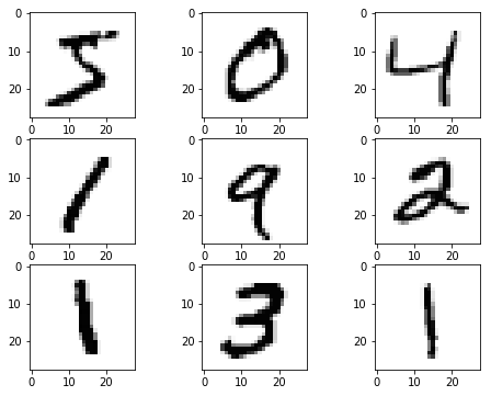
As a human I can eassilly recognize them as 5, 0, 4, 1, 9, 2, 1, 3, 1 (going by rows). But how can a computer do so?
# Loading the dataset
images, labels = load_mnist_data()
# Splitting it with a default 42 random state to be able to reproduce the results later
X_train, X_test, y_train, y_test = tts(images, labels, test_size=.8, random_state=42)
"""
    Here I am defining the predictor function, the classifier
    is an input parameter since any sklearn predictor or any other
    class that has a fit and a predict function that takes 2 and 1
    arguments of the relevant types can be passed to it.
"""

def predict(model, X_train, y_train, X_test):
    clf = model.fit(X_train, y_train)
    return clf.predict(X_test)
"""
    The confusion table represents the predicted accuracy
    of the model by showing the result distribution for each
    label. It is considered good if for all the labels the accuracy
    is the highest for the actual label, therefore the plot is mostly
    blue along the diagonal.
"""

def show_confusion_table(y_true, y_pred, labels, cmap=plt.cm.Blues):
    cm = confusion_matrix(y_true, y_pred, labels=labels)
    plt.figure(figsize=(7,7))
    plt.imshow(cm, interpolation='nearest', cmap=cmap)
    plt.title('MNIST')
    cm = cm.astype('float') / cm.sum(axis=1)[:, np.newaxis]
    plt.colorbar()
    tick_marks = np.arange(len(labels))
    plt.xticks(tick_marks, labels, rotation=45)
    plt.yticks(tick_marks, labels)

    fmt = '.2f'
    thresh = cm.max() / 2.
    for i, j in itertools.product(range(cm.shape[0]), range(cm.shape[1])):
        plt.text(j, i, format(cm[i, j], fmt),
                horizontalalignment="center",
                color="white" if cm[i, j] > thresh else "black")

    plt.ylabel('True label')
    plt.xlabel('Predicted label')
    plt.tight_layout()
    plt.show()
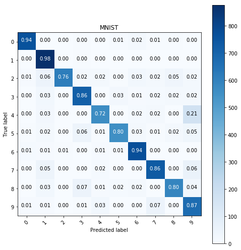
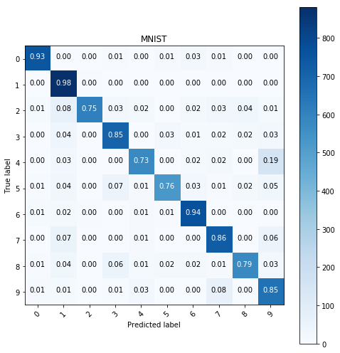
kNN
Using the weigthed kNN classifier with n=15 neighbors, the weights are the reciprocal distances and I used L2 metric. The results are shown below:
y_pred = predict(KNeighborsClassifier(n_neighbors=15, metric='l2', weights='distance'),
                 X_train, y_train, X_test)
show_confusion_table(y_test, y_pred, labels=range(10))

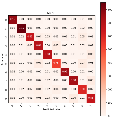
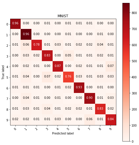
Multinomial logistic regression
Using multinomial logistic regression model, with L2 penalty the following results were acquired:
y_pred = predict(LogisticRegression(penalty='l2', multi_class='multinomial', solver='lbfgs'),
                X_train, y_train, X_test)
show_confusion_table(y_test, y_pred, labels=range(10), cmap=plt.cm.Reds)
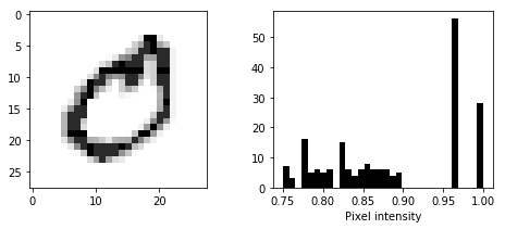
Histogram equalization
Histogram equalization ensures that images are more contrasty. It is a technique that transforms the images to achive better visibility. It is detailed here, however I am going to use a built in package from skimage.
from skimage import exposure
from scipy.stats import mode
def show_image_and_histogram(img):
    plt.figure(figsize=(8,3))
    plt.subplot("121")
    plt.imshow(img.reshape(28,28), cmap=plt.cm.Greys)
    plt.subplot("122")
    img_mode = mode(img).mode[0] # leaving out all the values corresponding to zeros
    plt.hist(list(filter(lambda x: x > img_mode, img.ravel())), bins=32, color='black')
    plt.xlabel('Pixel intensity')
show_image_and_histogram(exposure.equalize_hist(images[21]))
def build_eq_images_with_histos(images, bins=64):
    hists = []
    images_w_histos = []
    for img in images:
        img_mode = mode(img).mode[0]
        hist, _ = np.histogram(list(filter(lambda x: x > img_mode, img.ravel())), bins=bins, normed=True)
        eq_img = np.append(exposure.equalize_hist(img), hist)
        images_w_histos.append(eq_img)
    return np.array(images_w_histos).reshape(images.shape[0], images.shape[1] + bins)
equalized_images = build_eq_images_with_histos(images)
# Now splitting the equalized images
X_train, X_test, y_train, y_test = tts(equalized_images, labels, test_size=.8, random_state=42)
The images were equalized, the histograms were added to them with always leaving out the most common value from the histrogram creation when building the histograms. The bin size can be set through the bins parameter and now I shall go through the same process as before and I’ll compare the results.
# kNN algorithm with same parameters
y_pred = predict(KNeighborsClassifier(n_neighbors=15, metric='l2', weights='distance'),
                 X_train, y_train, X_test)
show_confusion_table(y_test, y_pred, labels=range(10))
# logistic regression model with same parameters
y_pred = predict(LogisticRegression(penalty='l2', multi_class='multinomial', solver='lbfgs'),
                X_train, y_train, X_test)
show_confusion_table(y_test, y_pred, labels=range(10), cmap=plt.cm.Reds)
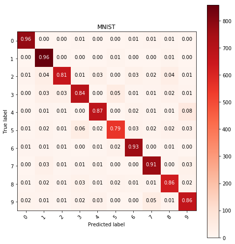
Histogram equalized images with edge detection
Using edge detection the result can be used as a feature of the image thus providing significant imformation on the image itself. I will be using edge detection provided as a feature of skimage.
from skimage.feature import canny
def build_eq_images_with_histos_and_edges(images, bins=64):
    hists = []
    images_w_histos = []
    for img in images:
        # Edge detection
        edges = canny(img.reshape(28, 28), sigma=0.8)*0.1
        img_mode = mode(img).mode[0]
        hist, _ = np.histogram(list(filter(lambda x: x > img_mode, img.ravel())), bins=bins, normed=True)
        eq_img = np.append(exposure.equalize_hist(img), hist)
        eq_img = np.append(eq_img, edges)
        images_w_histos.append(eq_img)
    return np.array(images_w_histos).reshape(images.shape[0], images.shape[1]*2 + bins)
eq_images_w_edges = build_eq_images_with_histos_and_edges(images)
# Now splitting the equalized images
X_train, X_test, y_train, y_test = tts(eq_images_w_edges, labels, test_size=.8, random_state=42)
# kNN algorithm with same parameters
y_pred = predict(KNeighborsClassifier(n_neighbors=15, metric='l2', weights='distance'),
                 X_train, y_train, X_test)
show_confusion_table(y_test, y_pred, labels=range(10))
# logistic regression model with same parameters
y_pred = predict(LogisticRegression(penalty='l2', multi_class='multinomial', solver='lbfgs'),
                X_train, y_train, X_test)
show_confusion_table(y_test, y_pred, labels=range(10), cmap=plt.cm.Reds)
Using the models
Using the previously described models with cross validation and extracting the diagonal elements of the confusion matrix to be able to compare them accurately:
images, labels = load_mnist_data(N=500)
def five_fold_cross_validate(model, images, labels, transform_function=None):
    cms = []
    if transform_function!=None:
        images = transform_function(images)
    for i in range(5):
        # Splitting
        X_train, X_test, y_train, y_test = tts(images, labels, test_size=.6, random_state=42*i+(137+i))
        clf = model.fit(X_train, y_train)
        y_pred = clf.predict(X_test)
        #show_confusion_table(y_test, y_pred, labels=range(10))
        cm = confusion_matrix(y_test, y_pred, labels=range(10))
        cm = cm.astype('float') / cm.sum(axis=1)[:, np.newaxis]
        cms.append(np.diag(cm))
    cms = np.array(cms).T
    mean_acc = np.mean(cms, axis=1)
    acc_std = np.std(cms, axis=1)
    return mean_acc, acc_std
acc0, std0 = five_fold_cross_validate(LogisticRegression(penalty='l2', multi_class='multinomial', solver='lbfgs'),
                        images, labels)
acc1, std1 = five_fold_cross_validate(LogisticRegression(penalty='l2', multi_class='multinomial', solver='lbfgs'),
                        images, labels, build_eq_images_with_histos)
acc2, std2 = five_fold_cross_validate(LogisticRegression(penalty='l2', multi_class='multinomial', solver='lbfgs'),
                        images, labels, build_eq_images_with_histos_and_edges)
It is evident from the results that the first, thus basic options seems to be the best for overall accuracy. The accuracy with edge detection turned on is better than only with histogram .
np.set_printoptions(precision=3)
print(acc0)
print('\t', std0) # logistic regression
print(acc1)
print('\t', std1) # logistic regression with histogram
print(acc2)
print('\t', std2) # logistic regression with histogram and edges
[0.935 0.913 0.762 0.83  0.886 0.655 0.92  0.838 0.707 0.825]
	 [0.05  0.009 0.076 0.05  0.056 0.106 0.022 0.056 0.042 0.058]
[0.85  0.959 0.713 0.824 0.848 0.483 0.876 0.736 0.656 0.704]
	 [0.088 0.013 0.092 0.097 0.073 0.077 0.046 0.092 0.025 0.097]
[0.88  0.964 0.743 0.818 0.848 0.523 0.884 0.781 0.664 0.751]
	 [0.077 0.014 0.087 0.055 0.064 0.081 0.044 0.079 0.015 0.103]
Loading the sofar unseen test data, but probably it is not much different than the previously seen training data, probably just artificially separated.
test_image = mnist.test_images()
test_labels = mnist.test_labels()
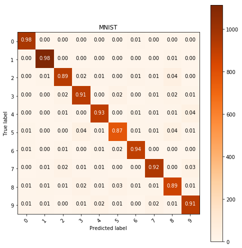
Basic logistic regression
images, labels = load_mnist_data(N=50000)
clf = LogisticRegression(penalty='l2', multi_class='multinomial', solver='lbfgs').fit(
    images, labels)
y_pred = clf.predict(test_image.reshape(test_image.shape[0], test_image.shape[1]*test_image.shape[2]))
show_confusion_table(test_labels, y_pred, labels=range(10), cmap=plt.cm.Oranges)
Logistic regression with equalization and histogram
clf = LogisticRegression(penalty='l2', multi_class='multinomial', solver='lbfgs').fit(
    build_eq_images_with_histos(images), labels)
y_pred = clf.predict(build_eq_images_with_histos(
    test_image.reshape(test_image.shape[0], test_image.shape[1]*test_image.shape[2])))
show_confusion_table(test_labels, y_pred, labels=range(10), cmap=plt.cm.Greens)
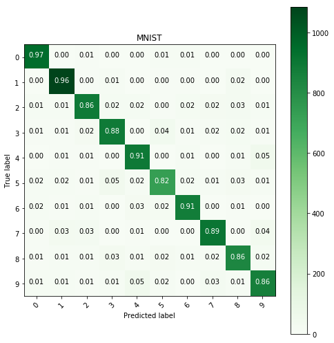
Generally it seems that the so called updated models perform worse than those that are just fitted with basic techniques.
@Regards, Alex

Alex Olar
Christian, foodie, physicist, tech enthusiast