
Photometric redshift summary
- 14 minsAbstract:
After reading several papers on the topic I had to reevaluate the methods that were used and test their accuracy and re-implement the majority of them.
Photometric redshift estimation is a highly popular area and is still very important today as a huge portion of the sky is not accurately measured or measured at all by spectroscopists so finding the redshift of available data and developing a good method and tool to accurately predict it would be highly beneficial for all.
My task is to get familiar with these concepts and try to find the best among them with machine learning techniques and general clustering algorithms.
The problem
The Sloan Digital Sky Survey has done an imaging survey in five optical bands which was later on followed by a spectroscopic measurement where more than a million galaxy was observed. The optical bands were matched with the right spectroscopic data and magnitudes and redshifts were calculated. It is all stored in a huge database which is available on the SDSS SkyServer [@server].
The magnitudes and petrosian magnitudes, which is corrected for each galaxy type and by other factors as well, can be found in this database with the appropriate errors and the spectroscopic data can be joined to it as well.
The database is a simple SQL database and scripts can be submitted to the CasJobs page on SkyServer to run and get the data from the servers. Therefore anyone has access to it freely and is able to do his/her experiments on it. I acquired most of my data by running this script:
    SELECT
  p.modelMag_u as m_u,
  ...
  p.modelMag_z as m_z,
  p.petroMag_u as pm_u,
  ...
  p.petroMag_z as pm_z,
  p.modelMag_u-p.extinction_u-p.modelMag_g+p.extinction_g as ug,
  ...
  p.modelMag_i-p.extinction_i-p.modelMag_z+p.extinction_z as iz,
  p.petroMag_u-p.extinction_u-p.petroMag_g+p.extinction_g as p_ug,
  ...
  p.petroMag_i-p.extinction_i-p.petroMag_z+p.extinction_z as p_iz,
  s.z as z into mydb.MyTable from PhotoObj AS p
  JOIN SpecObj AS s ON s.bestobjid = p.objid
WHERE
  p.probPSF=0 AND
  p.petroMagErr_u/p.petroMag_u BETWEEN 0 AND 0.05 AND
  ...
  p.modelMagErr_z/p.modelMag_z BETWEEN 0 AND 0.05
The WHERE clause states that I selected only galaxies from the SDDS DR7 database and all the acquired data have less then 5% error. This procedure resulted in 750’000 lines, although to run my simulations I only used a tiny bit of this in order to be able to make it run faster and handle errors in run time.
On this data set, I had to do the photometric redshift estimation. In order to do this I had to try different clustering algorithms myself and after that I had to move on with implementing the procedure from Róbert Beck’s article [@beck]. I got familiar with the problem by scanning through professor Csabai’s article [@csabai] and implementing some of the algorithms that could be found there and plotting the galaxy distributions by color indices.
Empirical methods
Approach
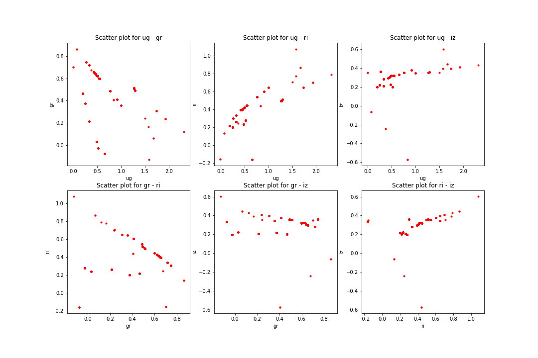
The acquired data was in .csv file format which can be easily read and processed by pandas package [@pandas] in . After reading the data I made the plots for model and petrosian magnitudes as well. The following figures will show the differences in color space:
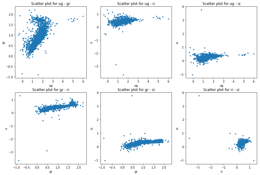
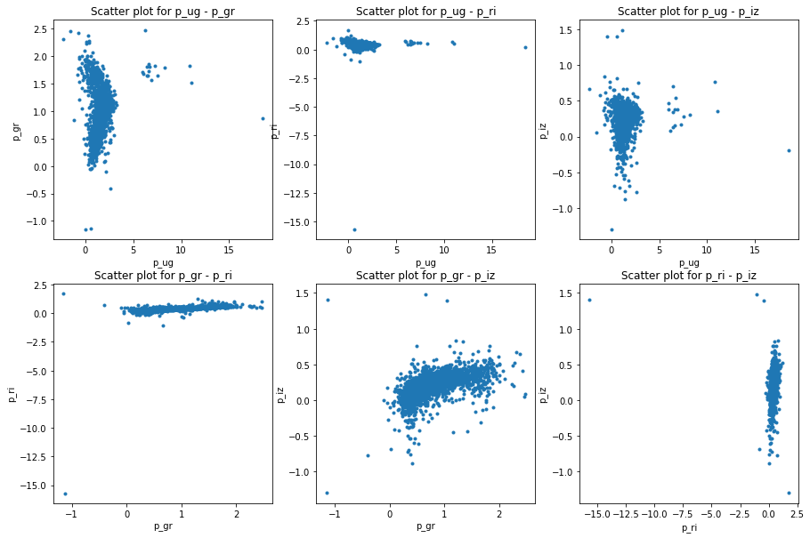
I consider this data as comparison baseline for the template data I have later on generated. Not only does the data need to cover the whole color space but also it should not contain too many outlier galaxies. This is taken care of as I only selected data points with small errors. A train-test split was done in 80%-20%.
Implementations, results
First of all I used a naive k-Nearest neighbor method. A brief introduction to the algorithm is the following: there’s a huge labeled dataset, the training dataset, with the appropriate color bands and redshift values. Using the test dataset we are looking for its k nearest neighbors and setting its redshift value to the mean of the nearest neighbors.
On the other hand, I mostly used the algorithms from the sklearn package [@sklearn] which includes KNN, support vector machine (SVM) and random forest algorithms, which are very well optimized and are using great tricks to store and handle data efficiently. For example, the KNN algorithm provided by sklearn used kd-trees, a data structure that is fast to search and build from training data, therefore it is fast do find the nearest neighbors of any given point after training the model.
For validation purposes the training and test sets are gathered from the same source and both have measured redshift values. Therefore I was able to generally say something about the goodness of my predictive models, by predicting the acquired and measured redshift values. Cross validation
Results are shown on the plots and values below:
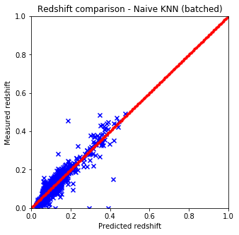
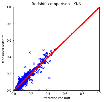
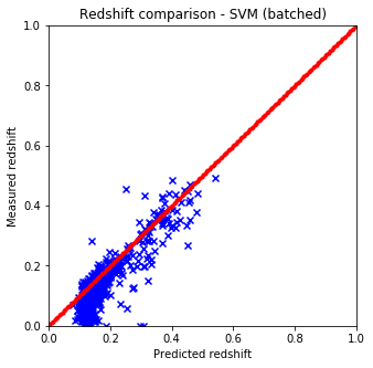
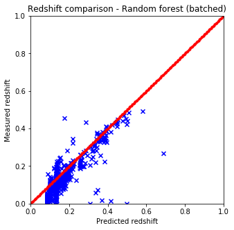
It is quite easy to see that the KNN algorithm is the best for the problem since the predicted redshift values for the training set fit well the measured redshift values of the training set. However, my naive KNN is way slower than the one provided by sklearn and needs to be batched for a huge input data file, thus gets worse and does not scale well. The support vector machine and the random forest algorithms does not predict redshifts very well for values lower than 0.15, thus later on I am going to use sklearn’s KNN.
Below a comparison can be seen for a five split cross validation for k = 7 nearest neighbors. For this purpose a ten thousand line 5% error limited data file was used.
| Method | MAE | MSE | Duration [s] |
|---|---|---|---|
| Random forest | 0.04296 +/- 0.00362 | 0.00850 +/- 0.00388 | 31.01 |
| Support vector machine | 0.05080 +/- 0.00328 | 0.00809 +/- 0.00322 | 1.07 |
| KNN | 0.02364 +/- 0.00127 | 0.00596 +/- 0.00348 | 2.28 |
| Naive KNN | 0.02364 +/- 0.00127 | 0.00596 +/- 0.00348 | 612.25 |
: Comparison of different algorithms on the example dataset
The best and worst values are presented in italics. It can be clearly seen that the best option is the KNN algorithm, using kd-trees from sklearn. It can be seen that without batching the naive KNN gives the same results but is much slower.
Local linear regression
Theory
According to the article of Beck [@beck] I was able to implement a local linear regression method by finding the k nearest neighbor of a test data point and fitting a linear function on those with the least-squares method. The process is the following: at first I needed to acquire the N \(\Big( = \frac{100}{166} \Big)\) nearest neighbors, secondly a least squares fitting must have been done, thirdly a prediction for the fitted nearest neighbors must be done to exclude the outlying values, finally the redshift must be predicted with the outlying values left out.
I am applying normalization on the data points as well, therefore, I am subtracting the mean of the data points and dividing by the standard deviation. This ensures that my data is correctly fitted and is less prone to rounding errors. The applied equations are the following:
\[\begin{align*} z_{pred, i} = c_{i} + \vec{a}_{i}\dot \vec{d}_{i} \\ \chi^{2}_{i} = \sum_{j \in NN} \frac{(z_{measured, j} - c_{i} - \vec{a}_{i}\dot \vec{d}_{j})^{2}}{w_{j}} \end{align*}\]Where, according to Beck d contains the r band and all the color indices ug, gr, ri, iz. The photometric redshift is predicted by doing a linear fit with the sklearn package by minimizing the \(\chi^{2}\) for each index.
After the fit the k nearest neighbors are gathered and they must be predicted with the local linear model. If their relative error calculated below is three times bigger, than the deviation of the predicted value, from the measured value, the fitted data point is dropped and the fit must be done again without the outlying neighbors. The weights (\(w_{j}\)) are all considered to be ones, however a weighted nearest neighbor algorithm can be fitted as well by using the standard \(\frac{1}{dist(point, data_{j})}\) weight metric.
\[\begin{align*} \delta z_{phot, i} \approx \sqrt{\sum_{j \in NN} \frac{(z_{measured, j} - c_{i} - \vec{a}_{i}\dot \vec{d}_{j})^{2}}{k}} \\ \Big| z_{measured, j} - c_{i} - \vec{a}_{i} \dot \vec{d}_{j} \Big| > 3 \dot \delta z_{phot, i} \end{align*}\]Results
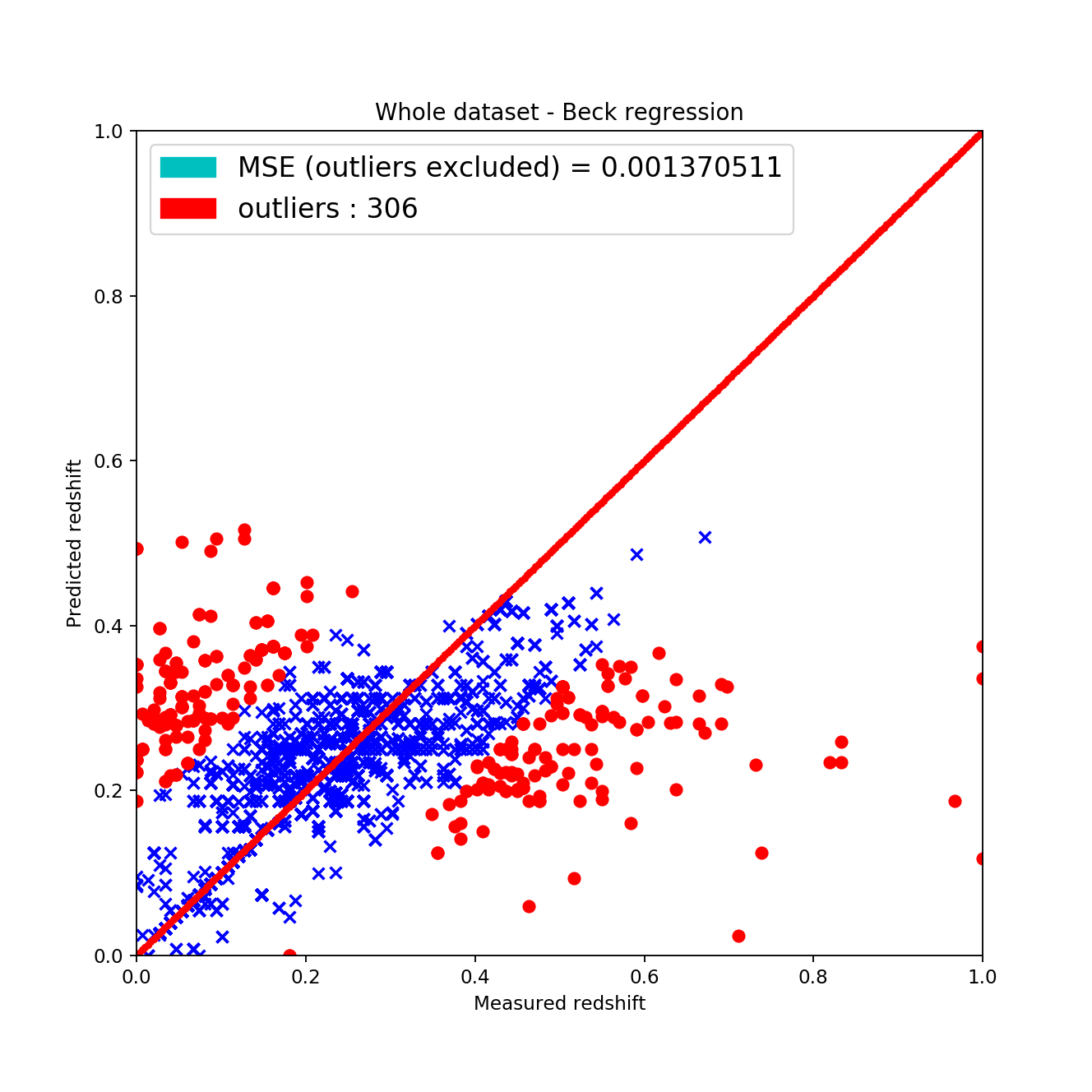
By implementing this algorithm I acquired the following results:
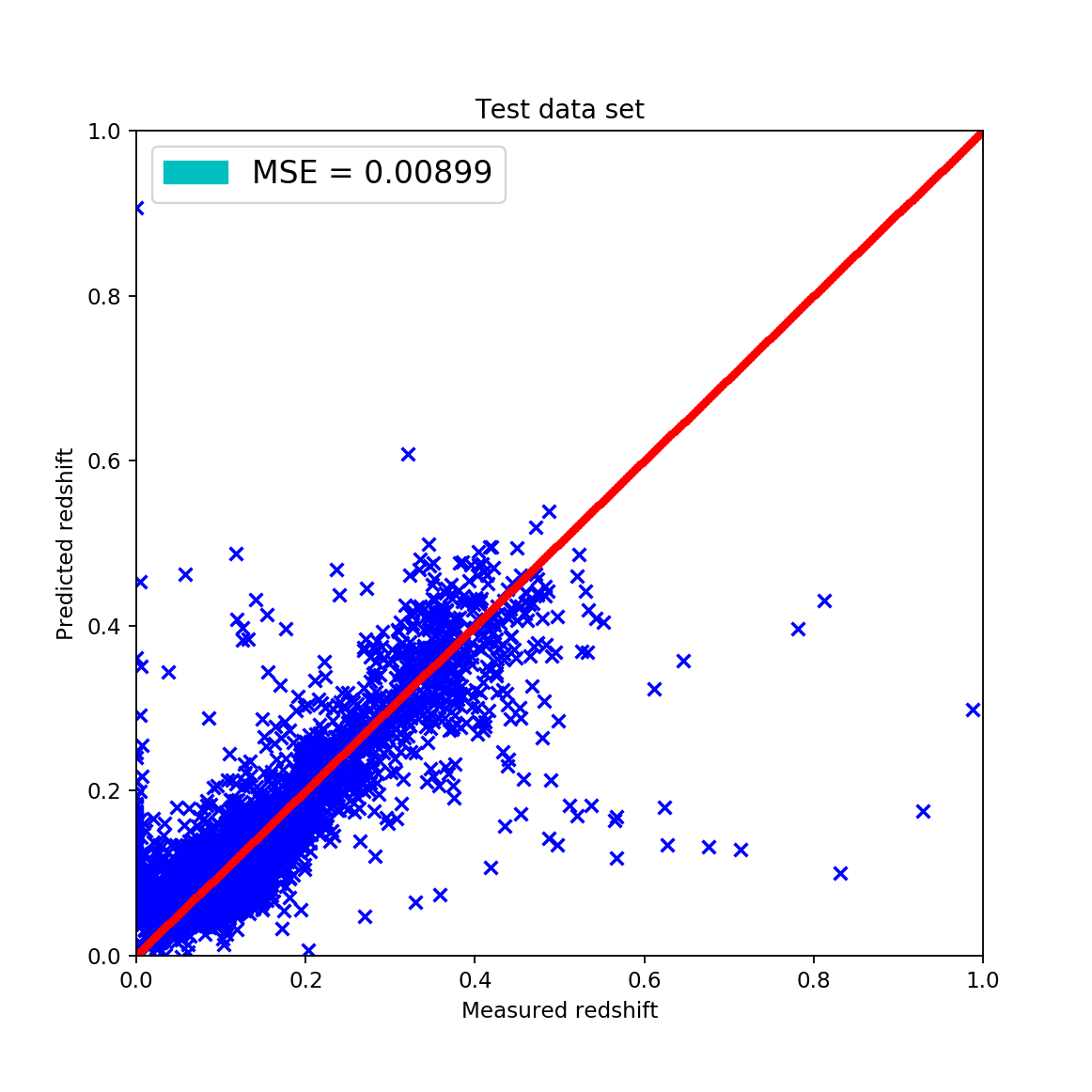
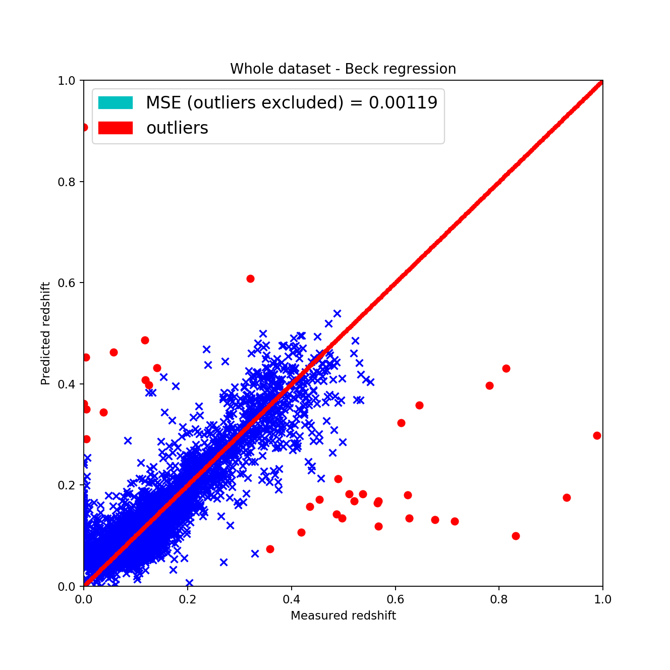
The train-test splits were made using a 20%-80% split by randomly shuffling the dataset for acquiring the most appropriate results. However, the fitted data can be qualitatively described by the these statements:
-
the wave-like shape has disappeared around the \(45^{\circ}\), \(z_{pred} = z_{measured}\) line this is considered good since it shows that the fit is actually showing signs of linearity
-
the mean squared error is approximately the same as with the KNN algorithm but after excluding the outliers it gets way better
-
analyzing the results of the cross validation it cannot be said that this approach is the best among all other since it isn’t the most stable regarding the standard deviations of MAE and MSE
| Method | MAE | MSE | Duration [s] |
|---|---|---|---|
| KNN | 0.02438 +/- 0.00035 | 0.00517 +/- 0.00011 | 12.12 |
| Beck’s method | 0.0267 +/- 0.00042 | 0.0069 +/- 0.00071 | 178.6 |
: Comparison of sklearn’s KNN and Beck’s local linear regression
The downside of the local linear regression fit is that is much slower than KNN, although that is not really considered bad since we have better computers and generally we don’t need fast algorithms, we need algorithms that finish in reasonable time and give the best results. It is very hard to say that the standard KNN algorithm is better since the scientific method gave a more linear result not by MAE or MSE but by pure reasoning according to the plots. (The cross validation was re-done for the KNN algorithm using the same 20%-80% split, shuffling and method.)
Template fitting
After completing the tasks above I headed to experiment with the so called template fitting where theoretical galaxy spectra is generated with different redshift values and best fits are selected compared to real, measured data points. This way it is possible to generate a model without having too many measured values. However, this method is considered much worse than the others above, and according to my calculations it is indeed much worse.
Photometric redshift is defined as:
\[\begin{align*} z = \frac{\lambda_{observed} - \lambda_{emitted}}{\lambda_{emitted}} \\ \lambda_{observed} = \lambda_{emitted}(1+z) \end{align*}\]Where the emitted spectrum is given from a template set. For this reason I used 299 spectrum files with wavelength and spectral value pairs. After applying the filters AB magnitudes had been calculated.
\[\begin{align*} F = \frac{\int S(\lambda)r(\lambda)\lambda d\lambda}{c\int r(\lambda)\frac{1}{\lambda}d\lambda} \end{align*}\]Whereas c is the speed of light \(S(\lambda)\) is the spectral function and \(r(\lambda)\) is the filter function which was acquired from voservices [@voservices]. Some of the selected spectral functions and all the filters are presented below:
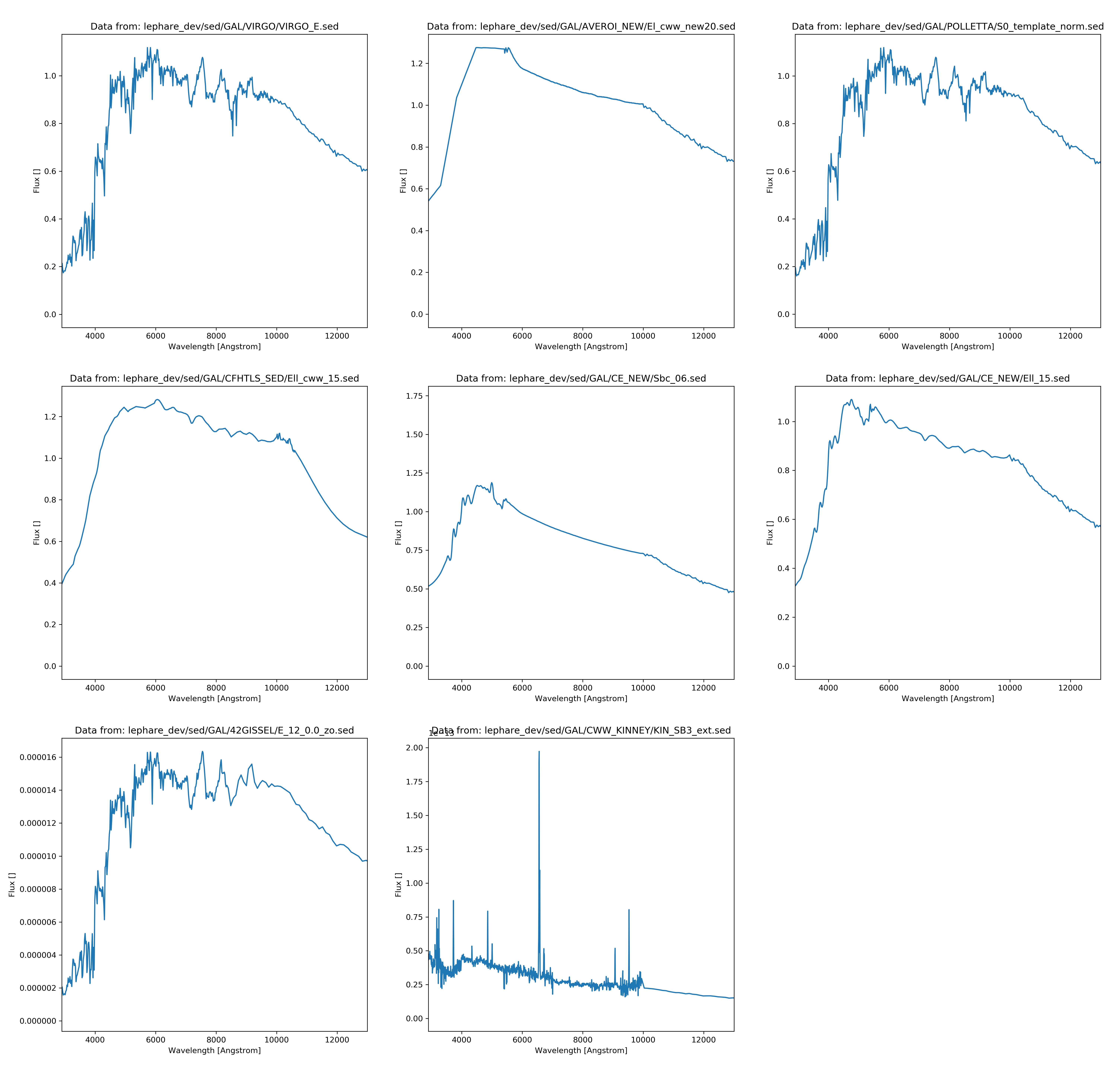
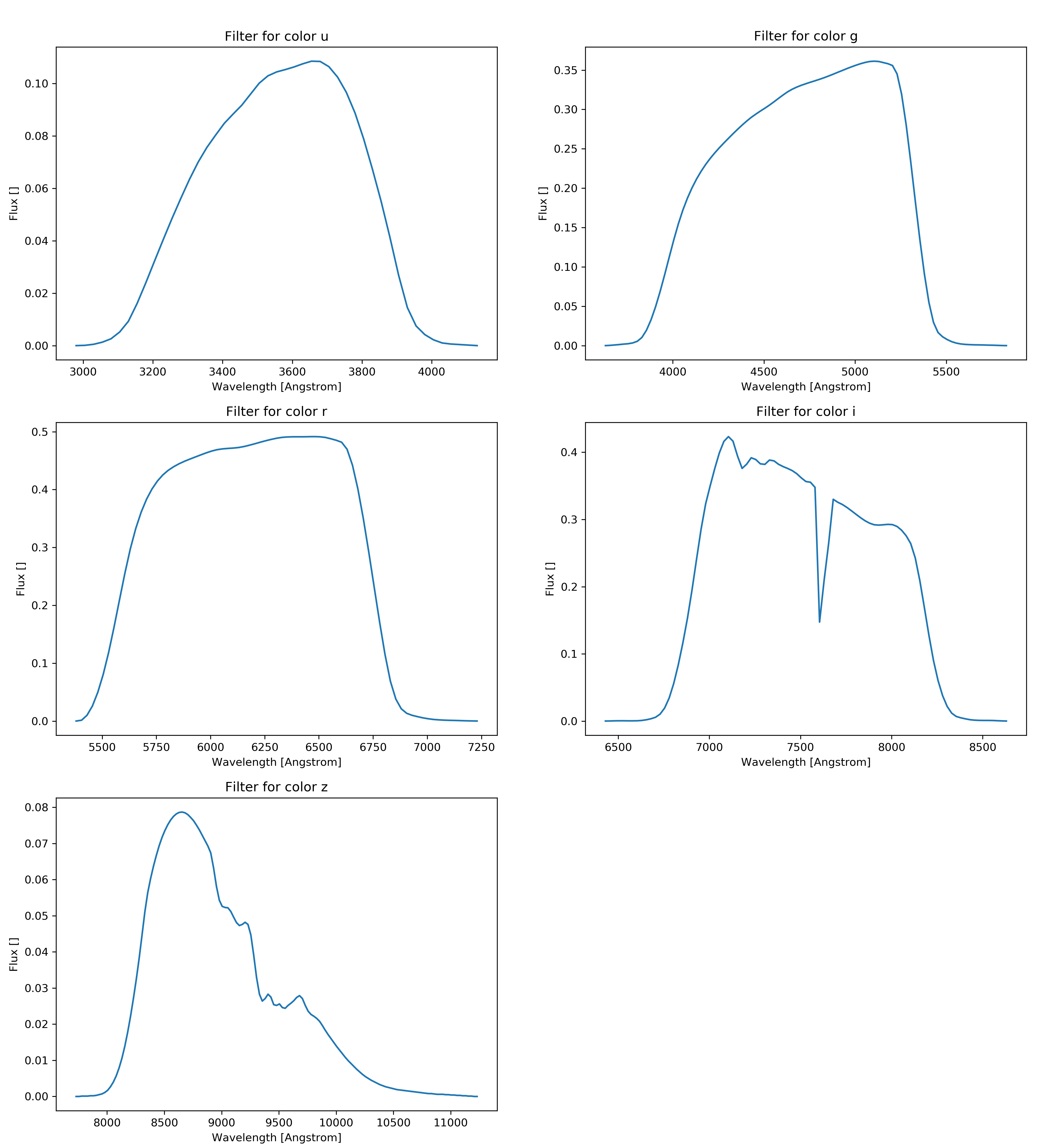
The AB magnitudes were calculated as:
\[\begin{align*} m_{ab} = -2.5 \dot log_{10}(F) - 48.6 \end{align*}\]For the integrals I used the following numerical method. I didn’t re-sample the data because I couldn’t find a general enough algorithm to do that so I wrote one. Firstly I looked for the minimum and maximum index of the nearest wavelength in the filters and in the spectral distribution. When that was found, I ran through that part of the spectral function and always multiplied the appropriate spectral value with the nearest filter-function value according to the wavelength. With this method I approximated the integrals and took into account that the wavelengths are in Angström.
from sklearn.neighbors import NearestNeighbors

def get_spectrum(spectrum, color_filter):
    # min/max wavelength
    min_lambda = color_filter[:,0][0]
    max_lambda = color_filter[:,0][-1]

    # find nearest min/max indices
    min_nearest_ind = np.abs(spectrum[:,0]-min_lambda).argmin()
    max_nearest_ind = np.abs(spectrum[:,0]-max_lambda).argmin()

    # integral of response function
    c = 3*10**8
    bin_width = color_filter[:,0][1] - color_filter[:,0][0]
    filter_integral = c*np.sum(color_filter[:,1]/color_filter[:,0])
    # dimension correction
    filter_integral *= 10**10

    flux = 0.

    # NN algorithm
    neigh = NearestNeighbors(n_neighbors=1, algorithm='kd_tree')
    neigh.fit(color_filter[:,0].reshape(-1, 1))

    for ind, val in enumerate(spectrum[:,0][min_nearest_ind:max_nearest_ind]):
        nearest_ind = neigh.kneighbors(np.array([val]).reshape(1, -1),
             return_distance=False)[0,:][0]
        delta_flux = color_filter[:, 1][nearest_ind]*spectrum[:,1][ind]*val
        # dimension correction
        delta_flux *= 10**(-10)
        flux += delta_flux
    return -2.5*np.log10(flux/filter_integral) - 48.60
The templates were acquired from the Le Phare [@lephare] dataset and most of the galaxy templates were used. I also acquired galaxy templates from Laszlo Dobos but I didn’t use them since they didn’t cover the whole wavelength spectrum, therefore it wouldn’t have been possible to return all color indices as the final goal of this process is to deduct the appropriate color indices with the matching redshift values.
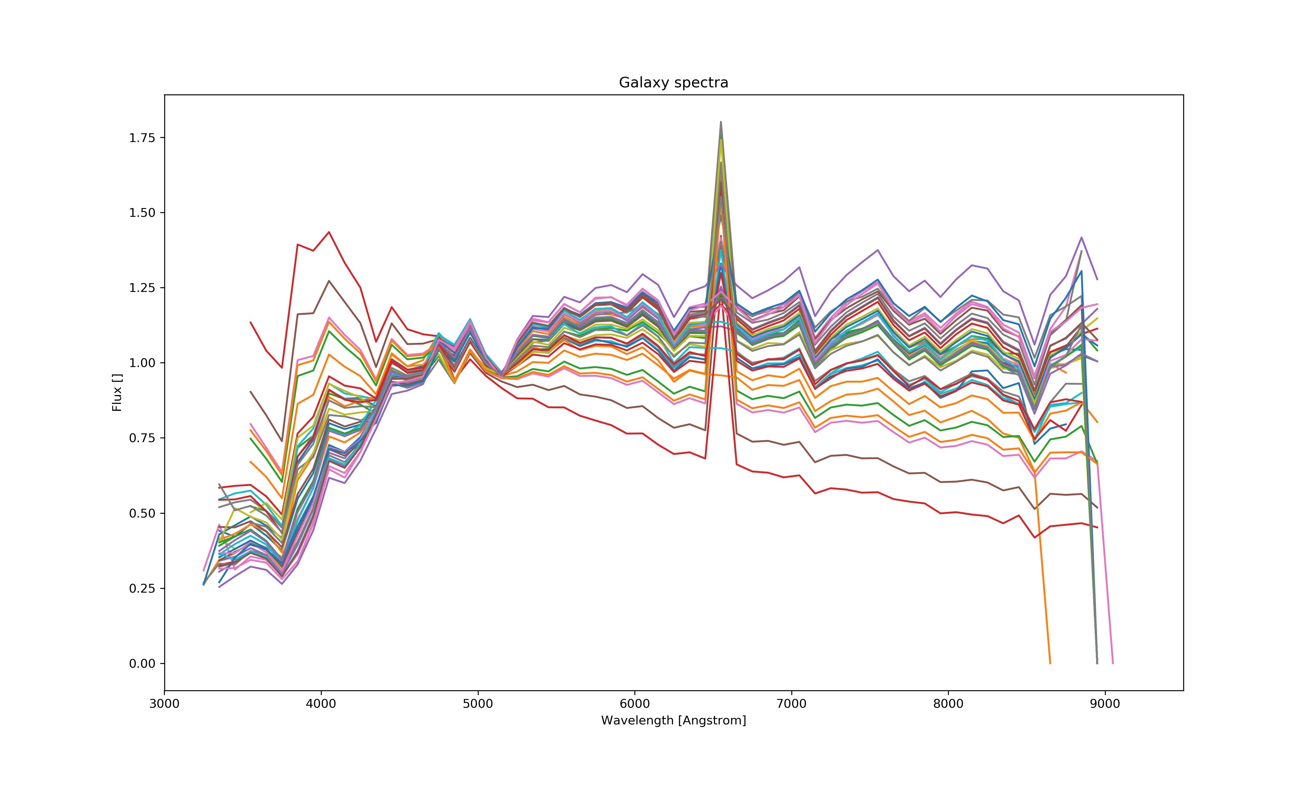
Using N dataset from Le Phare (N=299), applying the band filters (5) for each of them and setting a step size (step size = 150) for incrementing the redshift value the wavelengths were multiplied in each step and the color bands recalculated. This results in N*bands*step_size data points and thus much more calculations. This process was painfully slow therefore I was only able to generate at most 45 000 lines of template data and match less then half of it using ~ 800 000 lines of measured data.
The matching was done with KNN algorithm for the whole dataset line by line using sklearn therefore it was easy and fast to match even hugh amounts of data. Only a small portion of it (~ 20%) was selected for further process since most of the template data is junk and only some of it can be used as representative. The matching was done using the ug, gr, ri, iz color indices and the redshift value. However, as it can be seen below the matched data is not correct since it does not cover the whole color space. It is sometimes completely off, thus those data points are excluded since they only issue > 0.5% of the dataset.
It can be clearly seen that this is not the same as before for the measured data set and is not even close. It shows some resemblance to the petrosian data points but is objectively bad. Using a 20%-80% train-test split and excluding the completely off predictions the results are:

The matched set contained 12 000 points and around 9600 was used as test set. Approximately 3% of it contains outliers and > 0.5% is completely of by the predictor. The Beck method fails on the template set due to the fact that some points are amongst the points more than once and the linear regression can’t be done properly. Also a huge issue, that the data points do not cover the color space at all.
Overview
Therefore I completed all the tasks required to finish this project. I thinks that I made great progress throughout the weeks and I have overdone what I had to do. However, I am sure that there is some kind of problem with my template fitting as it has to be bad, but not this bad. My predictions are way off. All in all, I consider this work successful and I am happy that I could work on this. It raised my interest more to progress in the machine learning field further.
@Regards, Alex

Alex Olar
Christian, foodie, physicist, tech enthusiast