def knn_regression(x2pred, x_train, y_train, k=10):
    """Return prediction with knn regression."""
    return y_pred

import numpy as np
import pandas as pd
import matplotlib.pyplot as plt
import time

dataset = pd.read_csv("photoz_mini.csv")
print(dataset.columns.values)
colors = ['u', 'g', 'r', 'i', 'z']

# split u, g, r, i, z channels
sets = np.split(dataset.values[:,2:7], 5)
test = sets[0]
train = np.concatenate(sets[1:5])
# split redshifts
sets = np.split(dataset.values[:,7], 5)
test_redshift = sets[0]
train_redshift = np.concatenate(sets[1:5])
# get shapes
print(train.shape, train_redshift.shape)
print(test.shape, test_redshift.shape)

def knn_regression(x2pred, x_train, y_train, k=10):
    y_pred = []
    for dp in x2pred:
        dists = np.array([np.sqrt(np.sum(np.square(dp-value))) for value in x_train])
        ind = np.argpartition(dists, k)
        neighbors_redshift = y_train[ind][:k]
        y_pred.append(np.mean(neighbors_redshift))
    return np.array(y_pred)

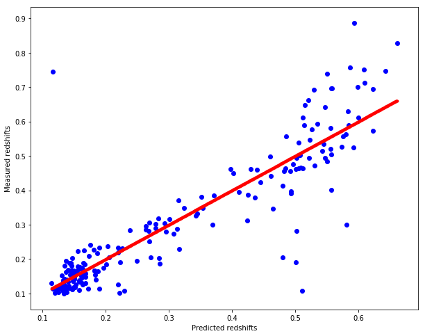
pred_redshift = knn_regression(test, train, train_redshift)
# Plot redshifts: predicted-valid
plt.figure(figsize=(10.,8.))
plt.scatter(pred_redshift, test_redshift, c="b")
plt.xlabel("Predicted redshifts")
plt.ylabel("Measured redshifts")
# Plot 45 degree line for grasping accuracy
x = np.linspace(np.min(pred_redshift), np.max(pred_redshift), num=1000)
plt.scatter(x, x, c="r", marker=".")

# get the mean squared error
MSE = np.sum(np.square(pred_redshift-test_redshift))/test_redshift.shape[0]
print("Mean squared error is %.5f" % MSE)

# get the mean absolute error
MAE = np.sum(np.absolute(pred_redshift-test_redshift))/test_redshift.shape[0]
print("Mean absolute error is %.5f" % MAE)

def cross_validate(algo, dataset, splits=5, k=10):
    MAEs = []
    MSEs = []
    start = time.time()
    for i in range(splits):
        # Sets for u, g, r, i, z indices
        sets = np.split(dataset[['u','g','r','i','z']].values, splits)
        x_test = sets[i]
        x_train = np.concatenate([st for ind, st in enumerate(sets) if ind != i])
        # Split for redshift
        sets = np.split(dataset['redshift'].values, splits)
        y_test = sets[i]
        y_train = np.concatenate([st for ind, st in enumerate(sets) if ind != i])
        y_pred = algo(x_test, x_train, y_train, k)
        MAEs.append(np.sum(np.absolute(y_pred-y_test))/y_test.shape[0])
        MSEs.append(np.sum(np.square(y_pred-y_test))/y_test.shape[0])
    print("Mean MAE : %.10f" % np.mean(MAEs))
    print("Standard deviation of MAE : %.10f" % np.std(MAEs))
    print("Mean MSE : %.10f" % np.mean(MSEs))
    print("Standard deviation of MSE : %.10f" % np.std(MSEs))
    end = time.time()
    print("The operation took %.5f seconds. " % (end-start))

cross_validate(knn_regression, dataset, splits=10, k=13)

from sklearn.neighbors import NearestNeighbors

def sklearn_knn_regression(x2pred, x_train, y_train, k=10):
    neigh = NearestNeighbors(n_neighbors=k)
    neigh.fit(x_train)
    y_pred = []
    for indices in neigh.kneighbors(x2pred, return_distance=False):
        y_pred.append(np.mean(y_train[indices]))
    return np.array(y_pred)

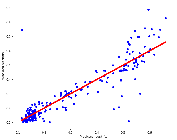
sklearn_pred_redshift = sklearn_knn_regression(test, train, train_redshift)
# Plot redshifts: predicted-valid
plt.figure(figsize=(10.,8.))
plt.scatter(sklearn_pred_redshift, test_redshift, c="b")
plt.xlabel("Predicted redshifts")
plt.ylabel("Measured redshifts")
# Plot 45 degree line for grasping accuracy
x = np.linspace(np.min(sklearn_pred_redshift), np.max(sklearn_pred_redshift), num=1000)
plt.scatter(x, x, c="r", marker=".")

cross_validate(sklearn_knn_regression, dataset, splits=5, k=7)

# I rerun this here just to have the values below each other.
cross_validate(knn_regression, dataset, splits=5, k=7)

def weighted_knn_regression(x2pred, x_train, y_train, k=10):
    y_pred = []
    for dp in x2pred:
        dists = np.array([np.sqrt(np.sum(np.square(dp-value))) for value in x_train])
        ind = np.argpartition(dists, k)
        neighbors_redshifts = y_train[ind][:k]
        neighbors_distances = dists[ind][:k]
        y_pred.append(np.sum(neighbors_redshifts/neighbors_distances)/np.sum(1./neighbors_distances))
    return np.array(y_pred)

weighted_pred_redshift = weighted_knn_regression(test, train, train_redshift)
# Plot redshifts: predicted-valid
plt.figure(figsize=(10.,8.))
plt.scatter(weighted_pred_redshift, test_redshift, c="b")
plt.xlabel("Predicted redshifts")
plt.ylabel("Measured redshifts")
# Plot 45 degree line for grasping accuracy
x = np.linspace(np.min(weighted_pred_redshift), np.max(weighted_pred_redshift), num=1000)
plt.scatter(x, x, c="r", marker=".")

cross_validate(weighted_knn_regression, dataset, splits=5, k=7)

def sklearn_weighted_knn_regression(x2pred, x_train, y_train, k=10):
    neigh = NearestNeighbors(n_neighbors=k)
    neigh.fit(x_train)
    y_pred = []
    distances, indices = neigh.kneighbors(x2pred, return_distance=True)
    for inds, dists in zip(indices, distances):
        y_pred.append(np.sum(y_train[inds]/dists)/np.sum(1./dists))
    return np.array(y_pred)

sklearn_weighted_pred_redshift = sklearn_weighted_knn_regression(test, train, train_redshift)
# Plot redshifts: predicted-valid
plt.figure(figsize=(10.,8.))
plt.scatter(sklearn_weighted_pred_redshift, test_redshift, c="b")
plt.xlabel("Predicted redshifts")
plt.ylabel("Measured redshifts")
# Plot 45 degree line for grasping accuracy
x = np.linspace(np.min(sklearn_weighted_pred_redshift), np.max(sklearn_weighted_pred_redshift), num=1000)
plt.scatter(x, x, c="r", marker=".")

cross_validate(sklearn_weighted_knn_regression, dataset, splits=5, k=7)