How does a recurrent neural network actually work? An implementation guide with detailed math

Recurrent neural networks

All blogs and books talk about recurrent neural networks when they mention sequence modelling. With recurrent networks it is possible to predict and generate sequences based on prior knowledge. The best architectures nowadays are the LSTM and the GRNN networks which are pretty similair to each other. The LSTM was developed decades ago and it is still provides exceptional results. A sequence can be a video, music, stock market exchange rates, but many other things can be read sequentially as well.

Andrej Karpathy sums up the basics about RNNs in this blog post of his and uses it to generate math articles in LaTeX, new baby names and does many other fun projects. I used his toy implementation a lot during implementing my simple RNN architecture and that can be found here in a nice and short gist.

The architecture

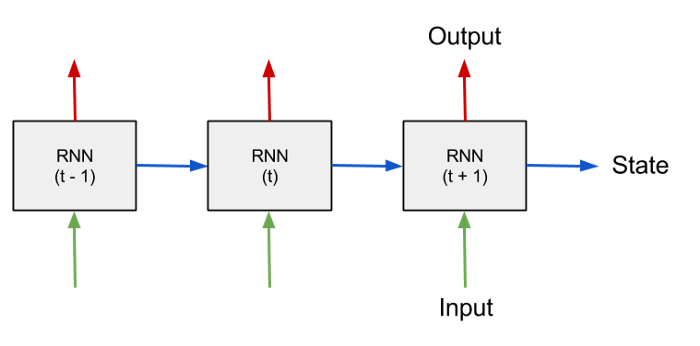
Where the RNN block in my case contains one hidden layer and works as follows:

Forward step

    def _foward_step(self, input):
        """
            input : must be one-hot encoded vocabulary_size vector
        """
        self.a = self.b + np.dot(self.W, self.h) + np.dot(self.U, input)
        self.h = np.tanh(self.a)
        self.o = self.c + np.dot(self.V, self.h)
        return np.exp(self.o) / np.sum(np.exp(self.o))

Basically there are three matrices \(W, U\) and \(V\) in this setup and two vectors \(\vec{b}, \vec{c}\) that need to be optimized in this task with back propagation through time (BPTT) . In a forward step we pass our input sequence’s element t : $\vec{x}^{(t)}$ to the model and and try to predict the next character \(\vec{\hat{y}}^{(t)}\) and update the state vector \(\vec{h}^{(t)}\) that propagates historic information forward in the system. The loss is defined as the negative loglikelihood read out at the target index (t.i.):

In recurrent networks t is called the timestep where t=1,…,T where T is the sequence length which is basically the number of recurrent steps that we unroll our RNN model for.

Backward step - back propagation

For backpropagation through time the model needs to know all previous activations, hidden states and output probabilities. Let’s start with the derivative of the loss function by \(\vec{o}^{(t)}\):

This is quiet simple to derive if we reduce the logarithm of the softmax function and derive by $\vec{o}^{(t)}$. The following steps are not that straightforward but can be calculated with some neat tricks. Using the chain-rule and applying the Einstein convention we need the following derivaties:

I am not going into detail about how to calculate these, but I’ll present the solutions here and if someone want to do the math he/she will have some kind of anchor to check. The point in back-propagation through time is that we need to do these updates backwards in time (the forward step we did a forward move through the sequence) and we need to accumulate the gradients that way:

Where \(\ast\) means piecewise multiplication.

    def _back_propagate(self, inputs, targets, probs, activations,
                        hidden_states):
        self.V_derivative = np.zeros_like(self.V)
        self.U_derivative = np.zeros_like(self.U)
        self.W_derivative = np.zeros_like(self.W)
        self.b_derivative = np.zeros_like(self.b)
        self.c_derivative = np.zeros_like(self.c)

        for ind in reversed(range(self.sequence_length)):
            loss_derivative = probs[ind]
            loss_derivative[targets[ind]] -= 1
            self.V_derivative += np.outer(loss_derivative, hidden_states[ind])
            self.c_derivative += loss_derivative
            db = np.dot(loss_derivative.T,
                        self.V).T * (1 - np.tanh(activations[ind])**2)
            self.b_derivative += db
            self.U_derivative += np.outer(db, inputs[ind])
            self.W_derivative += np.outer(db, hidden_states[ind - 1])

Optimization

Instead of Karpathy’s suggestion, at first I tried optimization with SGD. Well, it didn’t work, I needed to understand AdaGrad in order to be able to optimize properly and get low enough losses. AdaGrad basically accumulates previous derivatives into a memory and normalizes the current derivative with its value. I also apply gradient clipping to not let the gradients explode.

def _apply_gradients(self):
        ##########################################
        #########  Clipping gradients   ##########
        ##########################################
        np.clip(self.W_derivative, -1, 1, out=self.W_derivative)
        np.clip(self.U_derivative, -1, 1, out=self.U_derivative)
        np.clip(self.V_derivative, -1, 1, out=self.V_derivative)
        np.clip(self.b_derivative, -1, 1, out=self.b_derivative)
        np.clip(self.c_derivative, -1, 1, out=self.c_derivative)
        ##########################################
        #######     AdaGrad optiization    #######
        ##########################################
        self.memory_W += self.W_derivative ** 2
        self.memory_U += self.U_derivative ** 2
        self.memory_V += self.V_derivative ** 2
        self.memory_b += self.b_derivative ** 2
        self.memory_c += self.c_derivative ** 2
        self.W -= self.learning_rate * self.W_derivative / np.sqrt(self.memory_W + 1e-12)
        self.U -= self.learning_rate * self.U_derivative / np.sqrt(self.memory_U + 1e-12)
        self.V -= self.learning_rate * self.V_derivative / np.sqrt(self.memory_V + 1e-12)
        self.b -= self.learning_rate * self.b_derivative / np.sqrt(self.memory_b + 1e-12)
        self.c -= self.learning_rate * self.c_derivative / np.sqrt(self.memory_c + 1e-12)

ATTENTION : The forwards step code shown before applies the forward step in each timestep while backpropagation is done on the whole sequence at once as well as gradient update. The loss is set to zero after this and the whole optimization starts again from the current (updated) weights.

Data

I extracted some text from my fiancée’s blog:

Kedves,
Örülök, hogy rám találtál!
Van egy kócos nagy hajkoronám és sok mintás zoknim, hat testvérem és egy fekete nomád pulim, Bogár.
Budapesten tanulok - főleg élni, de ha valakit nagyon érdekel pegazus képzőn vagyok harmadéves...
Származási helyem Szerbia
Amikor megkérdezik, hogy mit szeretek csinálni, általában soha semmi nem jut eszembe, ezért egy ideje listát vezetek róla :bolyongani, idegenekkel spontán beszélgetni, enni, játszani, alkotni, hallgatni, bátornak lenni, győzni, levelet írni, mézeskalácsot díszíteni, Papával sétálni, ésatöbbiésatöbbi

Since sampling from the model is extremly straigh-forward I just copied the appropiate function from Karpathy’s blog and applied slight modifications to it:

    def _sample(self, seed_idx, sample_length=250):
        x = np.zeros((self.vocabulary_size, 1))
        x[seed_idx] = 1.
        seq = []
        h = np.zeros(shape=(self.hidden_size, 1))
        for t in range(sample_length):
            a = self.b + np.dot(self.W, h) + np.dot(self.U, x)
            h = np.tanh(a)
            o = self.c + np.dot(self.V, h)
            probs = np.exp(o) / np.sum(np.exp(o))
            idx = np.random.choice(range(self.vocabulary_size),
                                   p=probs.ravel())
            x = np.zeros((self.vocabulary_size, 1))
            x[idx] = 1.
            seq.append(idx)
        chars = [self.idx2char[idx] for idx in seq]
        return "".join(chars)

This samples 250 characters by default from the model and generates a sequence based on the text. The training interface is very neat and the following output is logged while training:

rnn = RNN(sequence_length, vocabulary_size)

char_to_idx = {ch: ind for ind, ch in enumerate(unique_chars)}
idx_to_char = {ind: ch for ind, ch in enumerate(unique_chars)}

data = {"chars": chars, "char_to_idx": char_to_idx, "idx_to_char": idx_to_char}

rnn.train(data, learning_rate=0.1)

Actual output:

Number of characters :  559
Number of unique characters :  44

>> Epoch : 1/100 	 Loss :  35.25008492296684
>> Sample : 
 ,, éatásen Palálniésstábaoésátálásépátesni,kélásni, hapávalásniöanagyőésásit sa
tálni, ésatöbbiésatöbbiésatöbitésat bésapöbtalábbit métölni, ésatöbbiésot l séta
lniésatöbbiésalálöiésatöbatásba satás sétaval sétésitösitálni,áésatöbbotáséaöiéz
átelasévaa 
>> Epoch : 2/100 	 Loss :  19.27816536135996
>> Sample : 
 otöbbii, sétálnibkésaltbbátalnatöésatöbalnibáétatöbbiélni, ésatöbbbolatalálés s
étálni, ésatöbbitánicsstöiálátani, Papövbalásatöbbi, é:val sétálatátát sétálni, 
ésatöbbibés sél sétálni, ésatöbbiélni, ésatöbbiésétöáni, éretk taésétöbbiísatöbá
tátétátbbib
...
...
...
>> Epoch : 98/100 	 Loss :  1.5867587438573225
>> Sample : 
  róla :bolyongani, alkotni, haláltál!
Van egy kócos nagy hal!
Van egy kócos nagy hajkoronám és sok mintás zoknim, hat testvérem érdekel pegazu
s képzőn vagyok harmadéves...
Származási hemegszélgképám, beszni, ésatöbbiésatöbbi, győzni, levelet írni, mé
>> Epoch : 99/100 	 Loss :  1.5652131199460997
>> Sample : 
  róla :bolyongani, alkotni, hallgatni, bátornak lenni, győzni, levelet írni, mé
zeskalácsot díszíteni, Papával sétálni, ésatöbbiésatöbbiésatöban soha sekelenni,
 győzni, bátornak li, hallgatni, győzni, levelet írni, mézeskalácsot díszíteni, 
Papával sét
>> Epoch : 100/100 	 Loss :  1.5065432739178304
>> Sample : 
  rólt e, egetni, enni, játornagyok harmadéves...
Származási helyem Szerbia
Amikor megkérdezik, hogy mit enni, játnten egy ideje listás zegezírnidelet írni,
 mézeskalácsot díszélgetni, enni, játszani, alkotni, hat ek mit szeretek, mit ír
ni, mézeskalács

Gibberish at the beginning but picks it up at the end and generates some pretty nice examples. It would be much more fun to do it on musical notes and generate music, ot stock market data to show the capabilities of such architecture but I didn’t have too much time to deal with those as well.

Obviously my implementation is not capable to handle large data. It is only a proof of concept and should not be used for actual tasks. All deep learning libraries have built in LSTM and GRNN modules already and are optimized heavily.

I hope you liked this little blog post, it took me an awful lot of time to think it through properly and to develop the code, which by the way, can be found here on my GitHub.

@Regards, Alex

Alex Olar

Christian, foodie, physicist, tech enthusiast

Tweet Share