Visualizing neural networks II.
- 19 minsVisualizing neurons, channels, layers…
All right, it seems that it is possible to train convolutional neural networks to classify, detect and segment objects. We also now that low lever filters might learn to detect edges, and that convolution was used before to do so, Sobel filters, Gabor filters all existed but deep learning provided a way not to hand engineer these feature detectors but to learn them from data. Maybe these aren’t even that great in the first place.
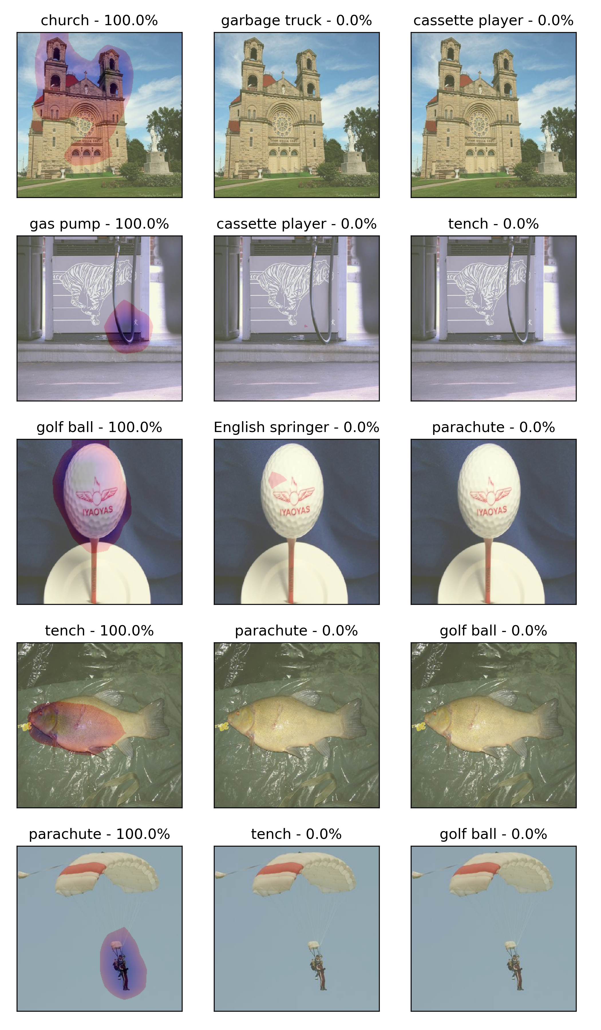
What might a high level neuron percept from the world? What might a channel see? These are all relevant questions since an awful lot of people are using CNNs as black boxes for some kind of freaky black magic.
In this distill article you can get a pretty nice overall understanding of the topic but with limited maths and actual implementation details. I digged into the provided resources from this article and checked-out the lucid library that is built on TensorFlow to visualize neural nets. I also did a simple re-implementation of all these algorithms with some of the tricky methods in order to make things look good.
Overview
Basically there are a limited number of ways to visualize ANNs. This picture provides the basic building blocks of feature visualization techniques:
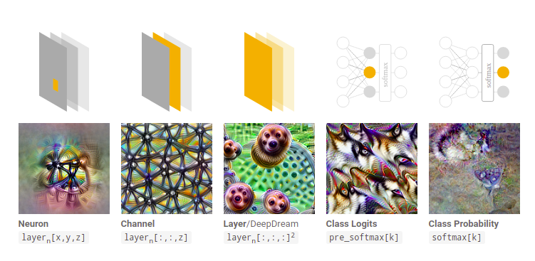
There is neuron-wise, channel-wise and ‘layer’-wise visualization as well as prediction-wise visualization. In all of these scenarios the objective is to maximize overall activation. The ‘layer’-wise or deepdream objective was hyped by Google since it produced very cool examples. I re-implemented in my code the loss function they use in their open-source guide.
Main idea
The main idea is that neural networks are chaining differentiable computations and therefore for each differentiable objective we could get the derivate of the input. For my visualizations I launch the network with a random noise input and try to maximize activations in a neuron/channels/a layer. Then I apply gradient ascent on the image and keep on going for a pre-defined number of steps. The image is updated every iteration but if you simple do this, nothing pretty will happen. You’ll get adversarial noise which added to an image can fool a neural network to predict something horribly wrong for a seemingly unchanged image.
Activation maximization
\[x^{*} = argmax_{x} f(x, \theta)\]Where f is the ANN and its parameters are all frozen since we are NOT trying to optimize the trained networks but the input image.
Tricks
It was discovered not long after adversarial examples that some kind of regularization techniques and transformations must be used to make the visualizations better. Scaling can produce scale-invariant features while rotating the images whilst optimizing it might produce rotation-invariant features. Applying a Gaussian-filter on the image blurs high-frequency features and reduces random noise. Padding the image might let information propagate to the edges while random jitter (cropping in random directions basically) helps with translation invariance. This is all theoretical as far as I understand and not quantitatively observed yet but sound promising and reasonable indeed.
Implementation
First I load the InceptionV3 model from tf.keras.applications with the imagenet weights. Then, as I above stated, I froze all layers and defined the models to get outputs from mixed2 and mixed4 layers. To make sure, I implemented assertion to test for 0 trainable parameters.
import tensorflow as tf
import tensorflow_addons as tfa
import tensorflow_probability as tfp
import tensorflow_addons as tfa
tfd = tfp.distributions

from IPython import display
import numpy as np
import matplotlib.pyplot as plt
inception = tf.keras.applications.InceptionV3(include_top=False, weights='imagenet')
for layer in inception.layers:
    layer.trainable = False

model = tf.keras.models.Model(inputs=inception.input,
                              outputs=[inception.get_layer('mixed2').output,
                                       inception.get_layer('mixed4').output])

assert len(model.trainable_variables) == 0, 'There should be no trainable variables.'
This Gaussian kernel was taken from stackoverflow but it is basically creating a 2 * size + 1, 2 *size + 1 2D Gaussian discrete function that is normalized. It is used to blur images and reduce noise.
def gaussian_kernel(size: int,
                    mean: float,
                    std: float,
                   ):
    """Makes 2D gaussian Kernel for convolution."""

    d = tfd.Normal(mean, std)

    vals = d.prob(tf.range(start = -size, limit = size + 1, dtype = tf.float32))

    gauss_kernel = tf.einsum('i,j->ij',
                                  vals,
                                  vals)

    return gauss_kernel / tf.reduce_sum(gauss_kernel)
Here I define the loss terms for each scenario that I tested. The deepdream_loss is a reduced sum over the reduced mean of several layer outputs. The single_node_loss is basically a reduce sum over 1 output value but it is needed since the shape might be not a scalar shape. Channel-wise I take the reduced mean.
def deepdream_loss(model_outputs):
    losses = []
    layer_activations = model_outputs
    for layer_activation in layer_activations:
        loss = tf.math.reduce_mean(layer_activation)
        losses.append(loss)
    return tf.reduce_sum(losses)

def single_node_loss(model_output):
    return tf.reduce_sum(model_output)

def single_channel_loss(model_output):
    return tf.reduce_mean(model_output)
The Gaussian kernel that I defined above should be applied to the image. Application means convolving it with the input image, but since we made a single channel filter we need to do the convolution on each channel with a new blurring kernel and concatenate the blurred channels into a blurred, noise-reduced image.
def apply_gaussian_blur(image, mean, sigma, kernel_size):
    channels = []
    for ch in range(image.shape[-1]):
        K = gaussian_kernel(size=kernel_size // 2, mean=mean, std=sigma)
        K = K[:, :, tf.newaxis, tf.newaxis]
        channel = tf.nn.conv2d(tf.expand_dims(image[..., ch], axis=-1),
                                     K, strides=[1, 1, 1, 1], padding='SAME')
        channels.append(channel)
    return tf.concat(channels, axis=3)
Here below the gradient step is implemented. Since Tensorflow 2, eager mode is activated by default, therefore if you want to do fast computations you need to use the @tf.function annotations. I won’t say I completely understand this Python magic here, I use the experimental_relax_shapes=True parameter since I got warnings without it for retracing. You also must make sure to use tf.constant default params in order to avoid retracing.
The logic here is that we take the gradient with respect to the the input and the loss function, then we normalize gradients and apply gaussian blur and gradient ascent on the image. After the gradient step we need to make sure that our input stays within the pre-defined boundaries that the network expects.
@tf.function(experimental_relax_shapes=True)
def make_step(x, model, loss_fn,
              step_size=tf.constant(1e-2, dtype=tf.float32),
              sigma=tf.constant(10, dtype=tf.float32)):
    with tf.GradientTape() as tape:
        tape.watch([x])
        y = model(x, training=False)
        loss = loss_fn(y)
        grads = tape.gradient(loss, x)
        # normalizing the gradients
        grads /= tf.math.reduce_std(grads) + 1e-8
        x = apply_gaussian_blur(x, 0, sigma, 3)
        x = x + grads * step_size
        x = tf.clip_by_value(x, -1, 1)
    return x
These code snippets are from the lucid library, they present random jitter with a pixel stride input, that basically does a random crop on the image and padding functions.
def jitter(d, seed=None):
    def inner(t_image):
        t_image = tf.convert_to_tensor(t_image, dtype=tf.float32)
        t_shp = tf.shape(t_image)
        crop_shape = tf.concat([t_shp[:-3], t_shp[-3:-1] - d, t_shp[-1:]], 0)
        crop = tf.image.random_crop(t_image, crop_shape, seed=seed)
        shp = t_image.get_shape().as_list()
        mid_shp_changed = [
            shp[-3] - d if shp[-3] is not None else None,
            shp[-2] - d if shp[-3] is not None else None,
        ]
        crop.set_shape(shp[:-3] + mid_shp_changed + shp[-1:])
        return crop

    return inner

def pad(w, mode="REFLECT", constant_value=0.5):
    def inner(t_image):
        if constant_value == "uniform":
            constant_value_ = tf.random_uniform([], 0, 1)
        else:
            constant_value_ = constant_value
        return tf.pad(
            t_image,
            [(0, 0), (w, w), (w, w), (0, 0)],
            mode=mode,
            constant_values=constant_value_,
        )

    return inner
The visualizer implements the gradient step for N_STEPS and uses octave scaling (up-scaling or down-scaling) on the image then does a full N_STEPS of optmization steps on the image. Jitter and padding is also applied by default and the blurring is changed each iteration. I didn’t implemented rotation due to the fact that the rotation operator in tensorflow-addons doesn’t seem to work currently.
N_STEPS = 200

def run_visualizer(x0, model, loss_fn, n_steps=N_STEPS, octave_scale=1.15, no_jitter=False, no_pad=False):
    x = x0
    sigma0 = 25.

    base_shape = x.shape[1:-1]
    float_base_shape = tf.cast(base_shape, tf.float32)

    for step in range(n_steps):

        octave_scale_factor = step // n_steps - 1
        new_shape = tf.cast(float_base_shape * octave_scale ** octave_scale_factor, tf.int32)
        if base_shape != new_shape:
            x = tf.image.resize(x, size=new_shape)

        if np.random.uniform() > .75 and not no_jitter:
            x = jitter(2)(x)

        if np.random.uniform() > .75 and not no_pad and step < 50:
            x = pad(3)(x)

        crt_sigma = tf.constant(sigma0 / tf.cast(step + 1, dtype=tf.float32))
        x = make_step(x, model, loss_fn, sigma = crt_sigma)
        if step % 9 == 0:
            IM = (x[0].numpy() + 1) * 127.5
            IM = np.clip(IM, 0, 255)
            IM = IM.astype(int)

            plt.imshow(IM)
            plt.xticks([])
            plt.yticks([])

            display.clear_output(wait=True)
            display.display(plt.gcf())
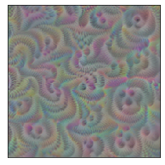
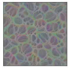
Here I use our previously defined mixed2, mixed4 layers output model with the deepdream_loss started from random normal noise, clipped to be within [-1, 1]. The output is pretty good, but joint optimization on different layers doesn’t really encode clear information.
x0 = tf.random.normal(shape=(1, 299, 299, 3), mean=0.0, stddev=1, name='input')
x0 = tf.Variable(tf.clip_by_value(x0, -1, 1))

run_visualizer(x0, model, deepdream_loss)
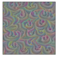
If I use random uniform distribution instead it doesn’t change the output much.
x0 = tf.random.uniform(shape=(1, 299, 299, 3), minval=-1., maxval=1., name='input')
x0 = tf.Variable(tf.clip_by_value(x0, -1, 1))

run_visualizer(x0, model, deepdream_loss)
For testing channel-wise loss I need to redefine the model:
for layer in inception.layers:
    layer.trainable = False

model = tf.keras.models.Model(inputs=inception.input,
                              outputs=inception.get_layer('mixed4').output[:, :, :, 42])

assert len(model.trainable_variables) == 0, 'There should be no trainable variables.'
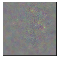
Channel wise loss:
x0 = tf.random.normal(shape=(1, 299, 299, 3), mean=0.0, stddev=1, name='input')
x0 = tf.Variable(tf.clip_by_value(x0, -1, 1))

run_visualizer(x0, model, single_channel_loss)
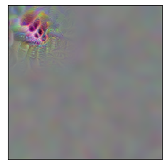
For neuron-wise loss, the redefinition was necessary as well. All the selected numbers are arbitrary here.
for layer in inception.layers:
    layer.trainable = False

model = tf.keras.models.Model(inputs=inception.input,
                              outputs=inception.get_layer('mixed4').output[:, 2, 2, 42])

assert len(model.trainable_variables) == 0, 'There should be no trainable variables.'

x0 = tf.random.normal(shape=(1, 299, 299, 3), mean=0.0, stddev=1, name='input')
x0 = tf.Variable(tf.clip_by_value(x0, -1, 1))

run_visualizer(x0, model, single_node_loss)
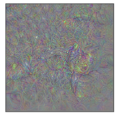
I went on and tested pre-softmax and softmax activation visualizations but I haven’t got very pretty results and I don’t know the reason yet. The acquire the pre-softmax activations or logits I needed to do the Dense computation by hand since Keras only provides the softmax outputs by default.
inception = tf.keras.applications.InceptionV3(weights='imagenet')

for layer in inception.layers:
    layer.trainable = False

model = tf.keras.models.Model(inputs=inception.input,
                              outputs=inception.get_layer('predictions').output[:, 0])

assert len(model.trainable_variables) == 0, 'There should be no trainable variables.'
Softmax visualization:
x0 = tf.random.normal(shape=(1, 299, 299, 3), mean=0.0, stddev=1, name='input')
x0 = tf.Variable(tf.clip_by_value(x0, -1, 1))

run_visualizer(x0, model, single_node_loss, no_jitter=True, no_pad=True)
def logodds_model():
    for layer in inception.layers:
        layer.trainable = False

    sub_model = tf.keras.models.Model(inputs=inception.input, outputs=inception.get_layer('avg_pool').output)

    weights, biases = inception.get_layer('predictions').get_weights()

    logodds = tf.add(tf.matmul(sub_model.output, weights), biases)

    model = tf.keras.models.Model(inputs=sub_model.input, outputs=logodds[:, 0])

    return model
Pre-softmax / logits visualization:
model_logodds = logodds_model()

run_visualizer(x0, model_logodds, single_node_loss, no_jitter=True, no_pad=True)
Conclusion
Here my goal was to understand the basic logic behind the different network visualization strategies and I think that I was able to do so. There are for sure some improvements to be made but for that there is lucid.
Regards, Alex

Alex Olar
Christian, foodie, physicist, tech enthusiast