Visualizing neural networks I.

Decision making in neural networks

This subject is loosely coupled with feature visualization since this is a visualization technique, however, it is not visualizing the neural network itself but the decision fields with a neat technique, that why it is now called attribution. GlobalAveragePooling is a technique used after convolutional layers to e.g. map an (None, 8, 8, 128) mapping to a (None, 1, 1, 128) mapping. Therefore it is creating a vector out of the last convolutional feature maps which can be fed to densely connected layers. This can also be done with GlobalMaxPooling or just flattening the last convolutional feature maps into a large vector but the downside of the former one is that CAM (class activation mapping) works best with average pooling and the former’s is its size. Flattening the last convolutional layer invokes creating a large matrix in the next layer of a densely connected network, thus increasing the number of parameters by a vast amount.

Class activation maps

Class activation maps were introduced in 2016 on a CVPR conference. The main idea is that based on the global average pooled vector and only one dense layer to make predictions we can calculate the importance of each feature map before pooling based on weights corresponding to classes predicted. Formalizing this mathematically:

Where W correspond to the matrix weights of the dense layer and we drop the bias term since for a large amount of parameters it really doesn’t matter that much. Moving on to the feature maps:

Where F is the feature map and we are doing multiplying each channel by a corresponding constant factor to get y. For each element of y we gat a class activation mapping (CAM) which we can visualize on top of the input image.

Implementation

Data

Tensorflow’s tensorflow-datasets API is providing us with a standard way of getting well-known datasets in .tfrecords format. This code will download imagenette which is a subset of the original ImageNet dataset with 10 pre-selected classes. Here I am downloading the training and validation sets.

imagenette = tfds.load('imagenette/320px', split=tfds.Split.TRAIN)
imagenette_validation = tfds.load('imagenette/320px', split=tfds.Split.VALIDATION)

Handling of the data is straight-forward. Since I am going to train a VGG19 model I am resizing each image to make both sides 320 pixels in height and width, while one-hot encoding the labels. I am applying VGG19 preprocessing on the images as well. After that I am creating a buffer of 15_000 elements (this fits all the data) and shuffling and batching it.

@tf.function
def apply_preproc(example):
    image, label = example['image'], example['label']
    image = tf.image.resize(image, [320, 320])
    image = tf.keras.applications.vgg19.preprocess_input(image)
    label = tf.one_hot(label, depth=10)
    return image, label

imagenette = imagenette.shuffle(buffer_size=15000).map(apply_preproc).batch(16)

imagenette_validation = imagenette_validation.shuffle(buffer_size=1500).map(apply_preproc).batch(8)

Moving on, I am creating the VGG19 model with a pre-defined input size of 320 x 320 x 3 applying the VGG19 model without the densely connected top/head and no pooling. I am then defining the GlobalAveragePooling layer to be able to extract the information and adding a Dense layer without bias and softmax activation to get predictions.

def create_model():
    input_image = tf.keras.layers.Input(shape=(320, 320, 3))
    vgg19 = tf.keras.applications.VGG19(weights='imagenet', input_shape=(320, 320, 3),
                                        include_top=False, pooling=None)
    
    x = vgg19(input_image)
    
    avg_pooled = tf.keras.layers.GlobalAveragePooling2D()(x)
    output = tf.keras.layers.Dense(10, activation='softmax', use_bias=False)(avg_pooled)

    model = tf.keras.Model(inputs=input_image, outputs=[output, avg_pooled, x])

    return model

Training is basically done by optimizing categorical cross-entropy with the Adam optimization algorithm and I am using a custom loop since the model outputs the predictions, the average pooling output and the feature maps before the average pooling since we are going to need that for the visualization.

optimizer = tf.keras.optimizers.Adam(lr=1e-5)
cce = tf.keras.losses.CategoricalCrossentropy()

model = create_model()

acc = tf.keras.metrics.CategoricalAccuracy()

for epoch in range(10):

    step = 0.
    rolling_loss = 0.0

    for images, labels in imagenette:
        with tf.GradientTape() as tape:
            pred_labels, _, _ = model(images)
            loss = cce(pred_labels, labels)
            acc(pred_labels, labels)
        grads = tape.gradient(loss, model.trainable_weights)
        optimizer.apply_gradients(zip(grads, model.trainable_weights))
        step += 1
        
        rolling_loss += loss

        if step % 50 == 0:
            print('Training loss (for one batch) at step %s: %s' % (step, float(loss)))
            print('Seen so far: %s samples' % ((step + 1) * 32))
            print('Accuracy : %.3f' % acc.result().numpy())

    print('\nEPOCH %d | Loss : %.3f' % (epoch + 1, rolling_loss))
    print('Accuracy : %.3f\n' % acc.result().numpy())
    
    model.save_weights('weights.h5')

Finally I am validating the model on the validation set as well, on which Iam going to try to make predictions and visualize the class activation maps:

acc.reset_state()

for images, labels in imagenette_validation:
    pred_labels, _, _ = model(images, training=False)
    acc(pred_labels, labels)

print('VALIDATION ACCURACY : %.2f%%' % (acc.result().numpy() * 100.))

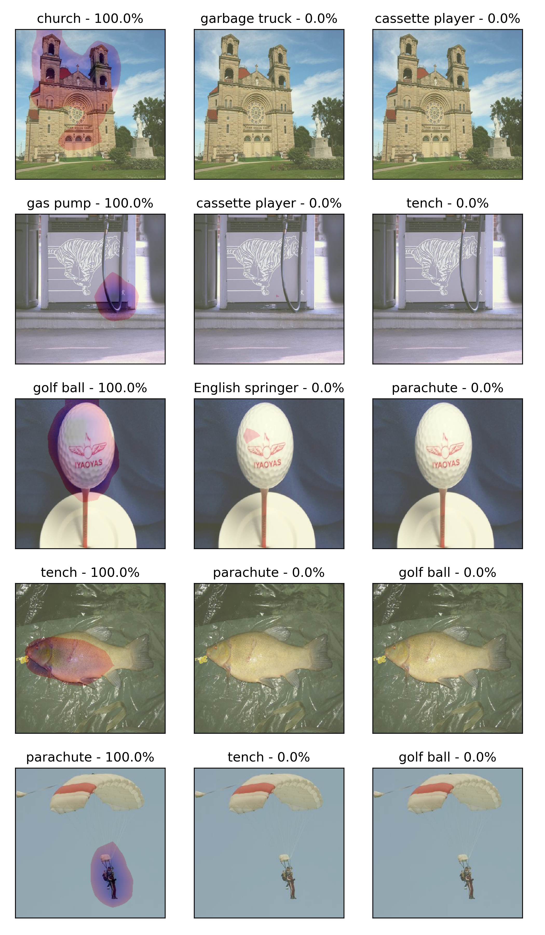
Moving on the the visualization of class activations we get the weights of the last layer (the Dense layer) of our model. Since it does not have bias it is just a matrix. Here I also created a list of all the classed in imagenette.

# Get weights from Dense layer
weights = model.layers[-1].get_weights()[0]

classes = ["tench", "English springer", "cassette player",
           "chain saw", "church", "French horn", "garbage truck", "gas pump",
           "golf ball", "parachute"]

We should not forget that we applied VGG19 preprocessing on our images which takes into account R, G, B mean pixel values on ImageNet and actually flips the RGB channels to BGR. So I applied de-processing on the input images before visualizing them.

vgg_means = [123.68, 116.78, 103.94]

for images, labels in imagenette_validation.take(1):
    
    pred_labels, avg_pooled, feature_maps = model(images, training=False)
    
    fig, axes = plt.subplots(5, 3, sharex=True, sharey=True, figsize=(7, 12))
    
    for img_ind in range(5):
        
        best_class = np.argmax(pred_labels[img_ind])
        
        BEST_MAP = feature_maps[img_ind] @ weights[:, best_class].reshape(feature_maps.shape[-1], 1)
        
        for ind, class_ind in enumerate(np.argsort(pred_labels[img_ind])[::-1][:3]):
            
            deprocessed_image = images[img_ind].numpy()
            deprocessed_image = deprocessed_image[..., ::-1] # BGR -> RGB
            for channel in range(len(vgg_means)):
                deprocessed_image[..., channel] += vgg_means[channel]
            deprocessed_image = deprocessed_image.astype(int)
            
            axes[img_ind, ind].imshow(deprocessed_image)
            class_weight = weights[:, class_ind].reshape(feature_maps.shape[-1], 1)
            
            CAM = (feature_maps[img_ind] @ class_weight)
            upsampled_cam = tf.image.resize(CAM, [320, 320]).numpy().reshape(320, 320)
            
            upsampled_cam /= np.max(BEST_MAP)
            upsampled_cam[upsampled_cam < .3] = .0
            
            axes[img_ind, ind].imshow(upsampled_cam, alpha=0.3, cmap="magma_r", vmin=.0, vmax=1., interpolation='bilinear')
            
            axes[img_ind, ind].set_title("%s - %.1f%%" % (classes[class_ind], 100. * pred_labels[img_ind, class_ind].numpy()))
            
            axes[img_ind, ind].set_xticks([])
            axes[img_ind, ind].set_yticks([])
        
        print('\n\n')
    fig.tight_layout()
    plt.savefig('heatmaps.png', dpi=300)

In detail: here I select the best prediction and I create the BEST_MAP variable in order to scale the less probable activation maps by the maximum of that. This is necessary to get prettier visualization and not to scale up noise, since the best map usually has larger activations due to the larger activation in the output neurons. After scaling the CAMs I also drop any part of the map that is less activated that 30%, this seems a reasonable choice. Since the CAM is as small as the output feature maps we need to upscale them to the original image size and then present.

Reproducibility

My code can be found on GitHub with the corresponding visualizations. Here I present only some examples:

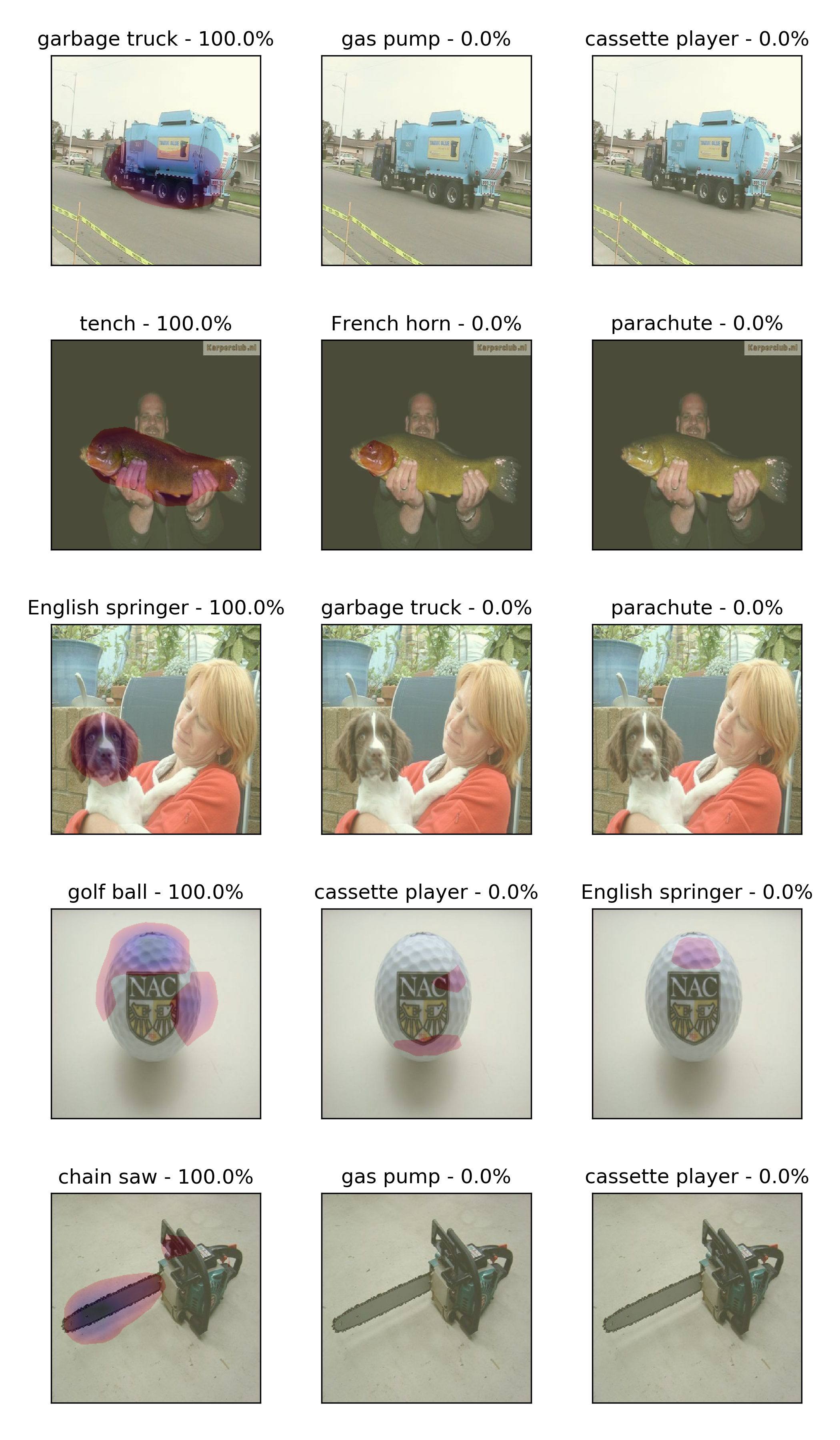
Above here, as it can be seen in the code above I visualized the three highest probability classes with their CAMs and they all present pretty well that the neural network makes decision from similar parts of the images as humans. We know the tench is a fish so we focus on the fish not the fisher. Trucks have several routes and usually a large body, etc.

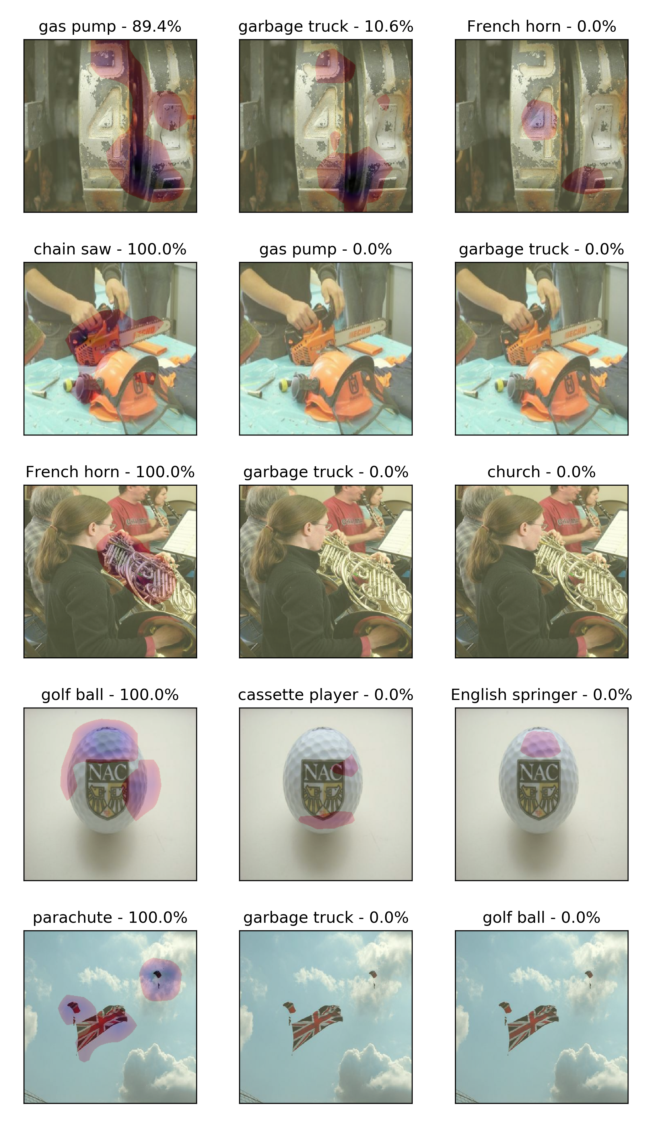
Sometimes the decision is not really straight-forward based on the image and when the confidence is lower we see parts of the image light up in CAM space. On the other hand, the parachute picture is pretty strong since the network focused on both persons in the sky.

Following

This post is part of a two-part series on NN visualizations, the next topic will present code for visualizing convolutional neural networks. I’ve read several papers on distill regarding this topic and I went on and reproduced some of the results to be able to see it my self what each neuron/layer/channel sees in a CNN.

@Regards, Alex

Alex Olar

Christian, foodie, physicist, tech enthusiast

Tweet Share