Autoregressive models - PixelCNN

Saturday. July 04, 2020 - 11 mins

+ deep learning + autoregressive models + pixelcnn + neural networks + mixture models

Autoregressive models - PixelCNN

An autoregressive model gives prediction on the next value based on all the previous values. In practice this means that given a sequence the probability of that sequence is a random sample from an underlying, assumed distribution for the first element and the next element then conditioned on the first and the third on the previous two and so on.

pixel-cnn-probability-assumption

For a rectangular image \(D = n^2\) and we need to impose raster scan ordering, meaning that we assume that the underlying generating process of the image is from top-to-bottom, left-to-right and R-G-B. This is rather non-intuitive but this is the way it was proposed and it seems to be working in PixelRNN/CNN, Conditional PixelCNN, PixelCNN++.

The aim of this network is to produce \(p(\textbf{x})\) from \(\textbf{x}\) and minimize the negative log likelihood by tuning its parameters with stochastic gradient descent. This was originally done with 256 softmax output for each color channel in PixelCNN. That is computationally non-effective so PixelCNN++ came up with a mixture of logistics (probability density) in order to ease computational constraints.

\[\nu = pixel\_{intensity} \sim \sum_{i = 1}^{K}\pi_i logistic(\mu_i, s_i) = \rho(\nu)\]

Where \(K\) is the number of probability densities while \(\mu_i, s_i\) are the parameters of the respective logistic densities and \(\pi_i\) are weighing constant that sum to \(1\) in order to make the logistic mixture a proper probability density function.

In PixelCNN++ they propose that for normal pixel values in the range of \(x \in [0-255]\) we should simply integrate the probability density around the actual pixel value. The choice of logistic functions is driven by the fact that they are analytically integrable therefore:

\[P_{\theta}(x) = \int_{x - \frac{1}{2}}^{x + \frac{1}{2}}\rho(\nu)d\nu = \sum_{i=1}^{K}\pi_{i}\Big( \sigma((x + .5 - \mu_i) / s_i) - \sigma((x - .5 - \mu_i) / s_i)\Big)\]

Where the neural network instead of 256 values for each color channel output \(N\_MIXTURES \cdot 3\) values per color channel corresponding to \((\pi_i, \mu_i, s_i)\). In practice \(5-10\) mixtures would suffice. They also propose that for extreme values \(0\) or \(255\) we should expand the integrals to \(-\infty\) and \(\infty\) respectively since real pixel distributions are high-tailed:

\[P_{\theta}(x \leq 0) = \sum_{i} \pi_i \sigma((x + .5 - \mu_i) / s_i)\] \[P_{\theta}(x \geq 255) = \sum_{i} \pi_i \Big(1 - \sigma((x - .5 - \mu_i) / s_i)\Big)\]

The original implementation is a fully convolutional network with several residual blocks and two types of different masks. The creation of these masks are probably the trickiest part. The main goal is to make the current pixel value unseen to the model. This can be done with masking convolutional kernels. The first type of mask is used during the first convolution from the input, it conditions R on nothing, G on R and B on R, G. The later convolutions can be conditioned on the resulting R, G, B channels. (RGB \(\rightarrow\) RRRGGGBBB \(\rightarrow\) RRRRRRRRRGGGGGGGGGBBBBBBBBB \(\rightarrow\) etc.) this way no output pixel has seen more than the previous pixels (the receptive field is actually triangular and there is some blind spot that was fixed in with GatedPixelCNN). I think here only code speaks:

def create_mask(kernel, mask_type):
    K, _, C_in, C_out = kernel.shape
    mask = np.zeros(shape=(K, K, C_in, C_out))
    mask[:K // 2, :, :, :] = 1
    mask[K // 2, :K // 2, :, :] = 1
    # mapping from e.g. : R, G, B to RRR, GGG, BBB
    assert C_in % 3 == 0 and C_out % 3 == 0,\
    'Input and output channels must be multiples of 3!'
    if color_conditioning:
        C_in_third, C_out_third = C_in // 3, C_out // 3
        if mask_type == 'B':
            mask[
                K // 2, K // 2, :C_in_third, :
                C_out_third] = 1  # conditioning the center pixel on R | R
            mask[K // 2, K // 2, :2 * C_in_third, C_out_third:2 *
                      C_out_third] = 1  # -ii- on G | RG
            mask[K // 2, K // 2, :, 2 *
                      C_out_third] = 1  # -ii- on B | RGB
        elif mask_type == 'A':
            """
                Only used for the first convolution from the RGB input.
                It shifts the receptive field
                to the direction of the top-left corner,
                successive applications would results in no
                receptive field in deeper layers.
            """
            mask[
                K // 2, K // 2, :C_in_third, C_out_third:2 *
                C_out_third] = 1  # conditioning center pixel on G | R
            mask[K // 2, K // 2, :2 * C_in_third, 2 *
                      C_out_third:] = 1  # -ii- on B | RG
    else:
        if mask_type == 'B':
            mask[K // 2, K //
                      2, :, :] = 1  # condition on center pixel

I also have an implementation but the negative log likelihood calculation is unstable, GitHub implementation.

More code

Mask creation which is the most intricate part of the CNN implementation was discussed above. The most complex part of the implementation would be the negative log likelihood calculation. Given the above equations we have the network to output the means \(\mu_i\), scaling factors \(s_i\) and mixture weights \(pi_i\). The output of the network for RGB images therefoe consist of these three parameters for each color channel and for K mixture of logistic functions. The output size is therefore \(3 * K * 3\). Here I’ll explain the negative log likelihood generation in detail:

def neg_log_likelihood(target, output, n_mixtures, input_channels=3):
    B, H, W, total_channels = output.shape
    assert total_channels == input_channels * 3 * n_mixtures, 'Total channels should be equal to input_channels * 3 times the number of mixture models. (RGB + pi, mu, s)'
    output = tf.reshape(output,
                        shape=(B, H, W, input_channels, 3 * n_mixtures))
    means = output[..., :n_mixtures]
    log_scales_inverse = output[..., n_mixtures:2 * n_mixtures]
    mixture_scales = output[..., n_mixtures * 2:]

    mixture_scales = tf.nn.softmax(mixture_scales, axis=4)  # last index
    scales_inverse = tf.math.exp(log_scales_inverse)

    targets = tf.stack([target for _ in range(n_mixtures)], axis=-1)

    arg_plus = (targets + .5 - means) * scales_inverse
    arg_minus = (targets - .5 - means) * scales_inverse

    normal_cdf = tf.reduce_sum(
        (tf.nn.sigmoid(arg_plus) - tf.nn.sigmoid(arg_minus)) *
        mixture_scales,
        axis=-1)
    underflow_cdf = tf.reduce_sum(tf.nn.sigmoid(arg_plus) * mixture_scales,
                                    axis=-1)
    overflow_cdf = tf.reduce_sum(
        (1. - tf.nn.sigmoid(arg_minus)) * mixture_scales, axis=-1)

    probs = tf.where(target < -.99, underflow_cdf,
                        tf.where(target > .99, overflow_cdf, normal_cdf))

    log_probs = tf.math.log(probs + 1e-12)

    return tf.reduce_mean(-tf.reduce_sum(log_probs, axis=[1, 2, 3])
                            )  # reduce to sum of negative log_likelihood

We should reshape the output of the neural network to get the parameters for each color channel. Therefore extract the means, the scaling factors and the mixture weights. The mixture weights should be scaled to sum to 1, therefore apply a softmax function on them. Afterwards just stack the targets on top of each other to subtract the means of the same shape and to scale them all with the appropriate scaling factore that I made an inverse to make the calculation somewhat stable. Afterwards we could calculate the above described pixel probabilities with using the targets and the network outputs as the logistics parameters’. For extreme pixel values (-1, 1 or 0, 255) I use the appropriate probabilities with tf.where. Afterward I take the log of all probabilities and sum them on all the pixel values and mean them for the batch, take the negative and return it as the negative log likelihood on the batch.

Results

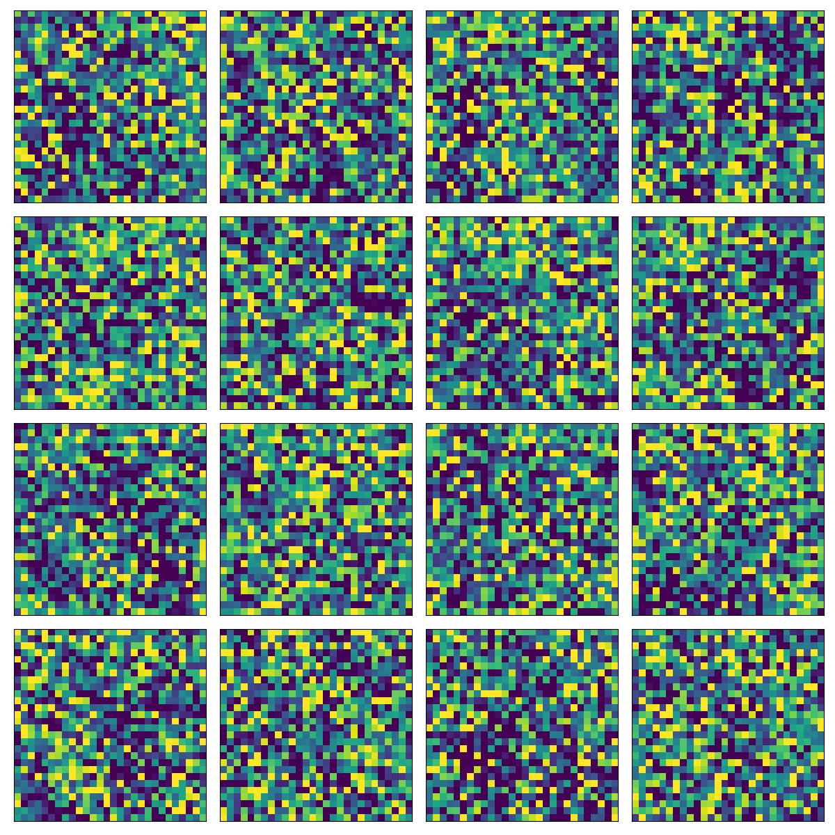
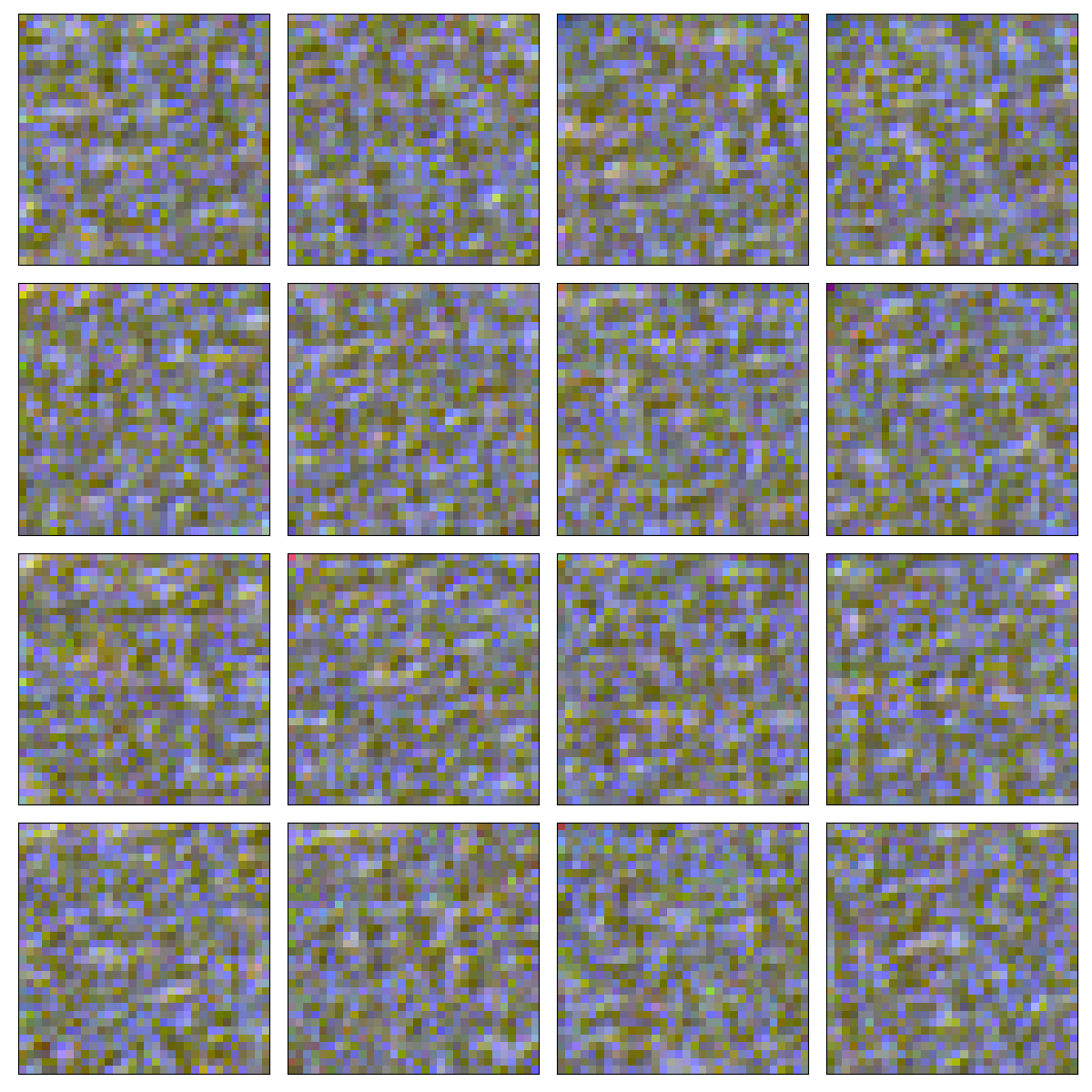
I ran myimplementation on the MNIST dataset and the CIFAR10 dataset. It does not produce any meaningful representations but at least it is minimizing the negative log likelihood to some extent. Since my implementation is not stable I needed to carfully tune the hyperparameters and I could fully optimize the models trained on either of the datasets. The results here by no means good but at least it can be seen that they are sensical:

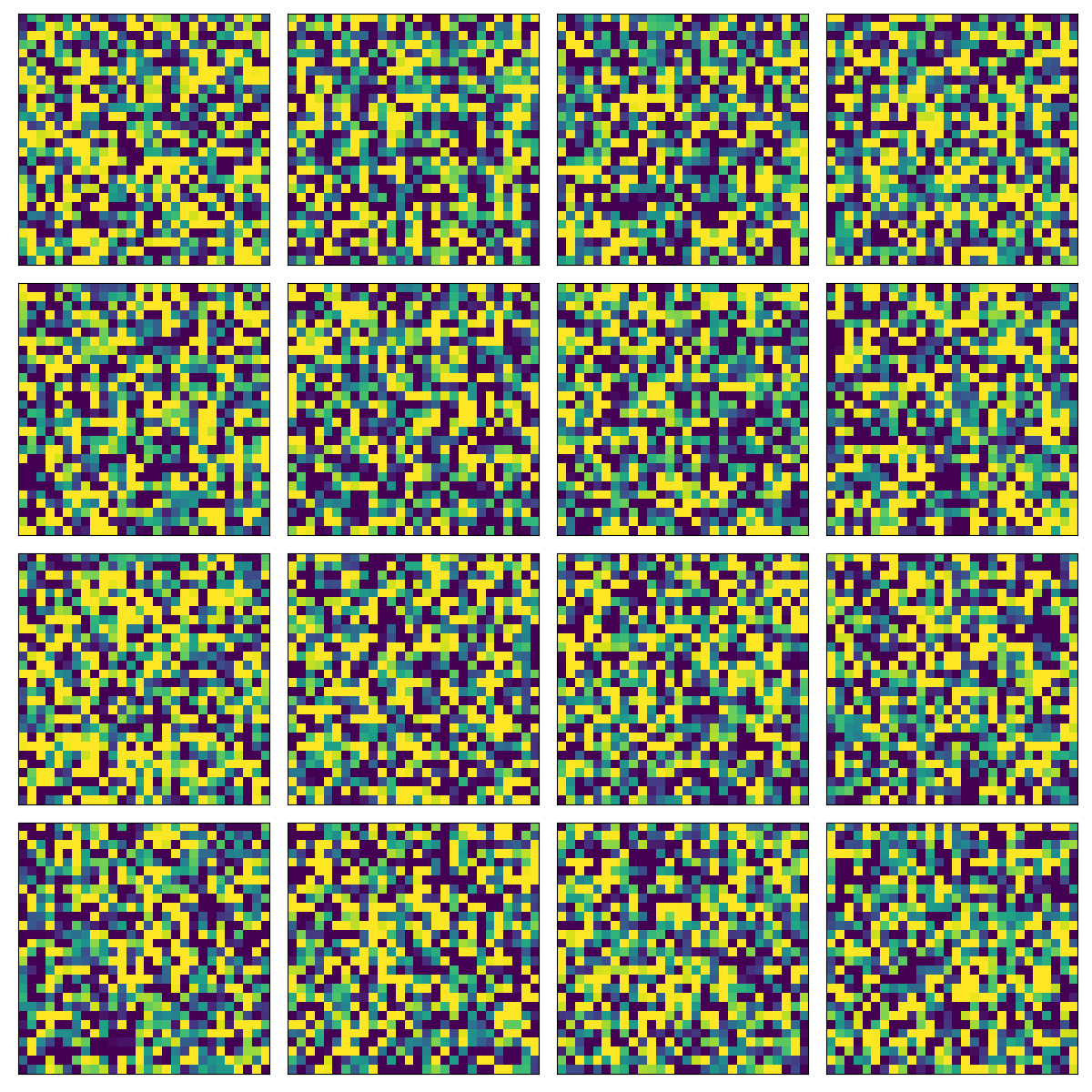
sampled-mnist-pixels-from-trained-model

sampled-cifar10-pixels-from-trained-model

This is actually not very good since optimization could not go very far. So I used the loss implementation from the OpenAI PixelCNN++ GitHub repository and upated it in order to work with Tensorflow 2. Luckily it was pretty easy to integrate with my code as it expected targets and outputs the same way I created my loss function. The only difference was the number of mixture models used and there is some confusion between the loss implementation and my code regarding the naming scheme. Using the OpenAI loss for training but the same sampling method with tensorflow_probability.distributions.Logistic (which is way easier that the sampling method used in the PixelCNN++ implementation):

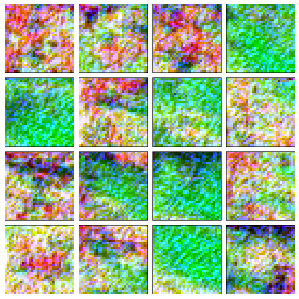
sampled-mnist-pixels-from-trained-model

sampled-cifar10-pixels-from-trained-model

The sampling method is using raster-scan-ordering, meaning that we go from top-to-bottom, left-to-right and from R, to G, to B starting from a random uniform pixel distribtuion and sampling the image pixel-by-pixel. It is extremely counter-intuitive but it seems to work pretty well in the VQ-VAE in order to generate photorealistic images.

Conclusion

I came across this paper and the concept more than 6 months ago but I finally understood it. I didn’t occupy with it for months but to build up the intuition and the necessary background from unsupervised learning took some time fur sure. I hope it helps out others as well to read this essay on the PixelCNN network and its implementation.