Hamiltonian neural networks

Hamiltonian neural networks

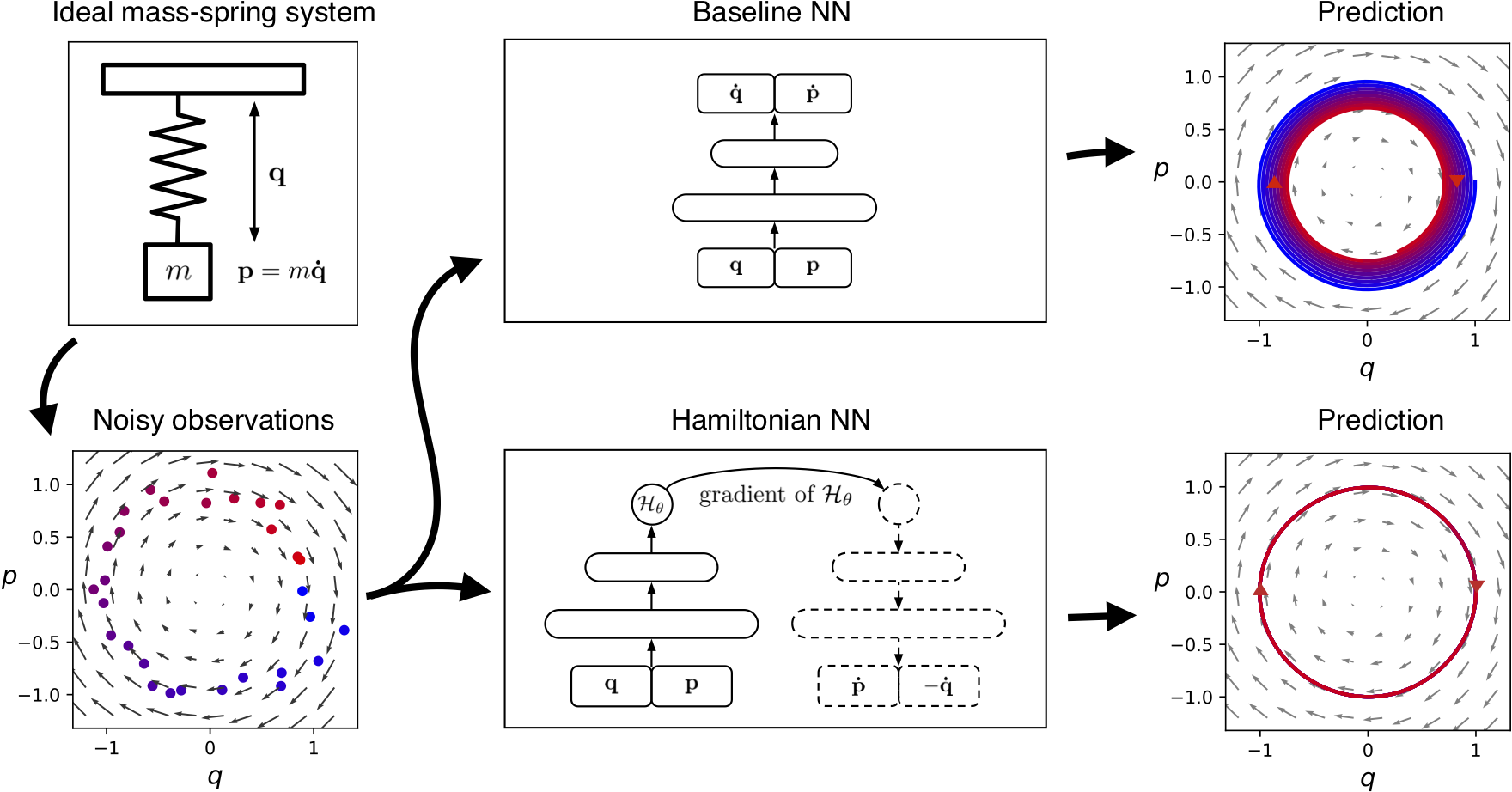
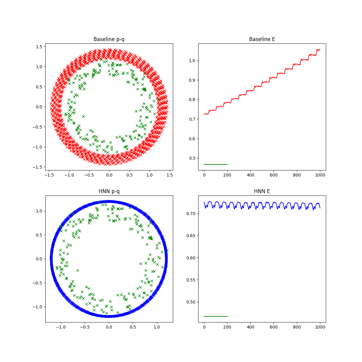
Recently I have found an article on Hamiltonian neural networks. The idea is very simple and neat: why don’t we apply the laws of Hamiltonian mechanics to a system and try to learn that instead of the next physically feasible frame/time step. Generally we can have a time point (x, y coordinates for example) and try to predict the next time point based on that. Training a neural network for this task is reasonably straight forward since we would only need enough training data - pairs of previous and next coordinate pairs - in order to achieve great results. However, the problem with these approaches is that they usually do not conserve energy very well since they cannot learn for previous and current data pairs that in a conservative system energy is conserved. Therefore the error of prediction adds up if we want to enroll the system and check its time evolution therefore loosing or gaining energy in each consecutive time step.

In Hamiltonian mechanics we have the Hamiltonian-function - H - which for which the following equations are true:

Where p, q are so called canonical coordinates. Therefore the Hamiltonian-function provides differential equations on the time evolution of the system by stating these two equations above that hold for the canonical impulse - p - and the canonical location - q - for all times in a conservative system.

Experiment

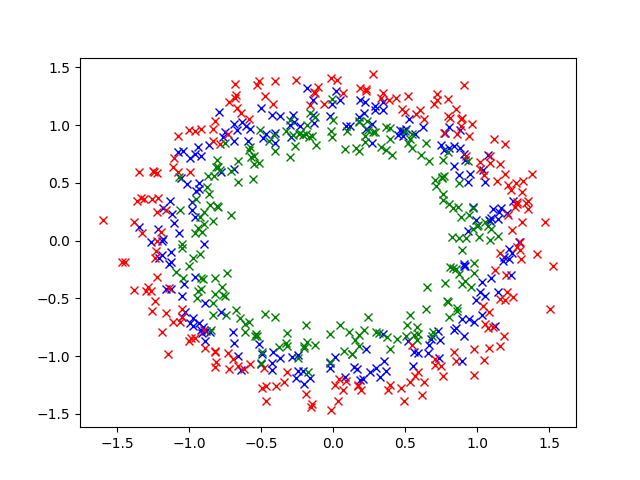
I went and reproduced the easiest experiment from the original article. I generated randomly (x, p) pairs of data points based on spring motion with k = m = 1 constants for simplicity.

The Hamiltonian is therefore very easy and the Euler-Lagrange-equations are the following:

These equations provide us with the derivatives of the (x, p) pairs for each time point and therefore we are able to generate new data points based on these with an RK4 differential equation solver algorithm.

def mass_spring_diff_eq(t, vec):
    x, p = vec
    return [p, -x]

In the article they generated data points with energy ranging in an interval [energy_low, energy_high] therefore this is what we did as well:

E = np.random.uniform(energy_low, energy_high)
phi = np.random.uniform(0, np.pi)
r = np.sqrt(2. * E)
x = r * np.cos(phi)
p = r * np.sin(phi)
sol = solve_ivp(mass_spring_diff_eq, t_span=[0, 100], y0=[x, p], first_step=0.1, max_step=0.1)

Here we used that the energy already defines the range of (x, p) on a circle therefore if we generate a random angle we can calculate x and p accordingly. Moving on we called the solve_ivp method from the scipy package. The default solver for this method is an adaptive RK4. After trajectory generation the some random noise is added to the data points following the ratio described in the article.

The neural network of choice is a simple MLP backbone. The MLP is used as a baseline for next time point generation and in the Hamiltonian neural network as well. But what is a Hamiltonian neural network?

Hamiltonian neural network

A Hamiltonian neural network relies on the fact that the Euler-Lagrange-equations must hold. The loss term of such a system tries to minimize the difference between the two parts of the EL-eqs by predicting the Hamiltonian-function, taking its derivatives and applying gradient according to the derivatives instead of the actual output.

The loss is therefore:

By applying gradient to the Hamiltonian network we try to minimize this quantity and therefore the system will intrinsically conserve energy if the loss is correctly minimized.

Technical details

The MLP backbone is very simple and is used as a baseline with two outputs for (x, p) -> (x_next, p_next) and with one output for the Hamiltonian net:

import torch


class MLP(torch.nn.Module):
    def __init__(self, output_dim = 2):
        super(MLP, self).__init__()
        self.mlp = torch.nn.Sequential(torch.nn.Linear(2, 128),
                                       torch.nn.Tanh(),
                                       torch.nn.Linear(128, 64),
                                       torch.nn.Tanh(),
                                       torch.nn.Linear(64, 32),
                                       torch.nn.Tanh(),
                                       torch.nn.Linear(32, output_dim, bias=None))

    def forward(self, x):
        return self.mlp(x)

For the Hamiltonian net:

import torch
from mlp import MLP

class HNN(torch.nn.Module):
    def __init__(self):
        super(HNN, self).__init__()
        self.mlp_backbone = MLP(output_dim=1)

    def forward(self, x):
        H = self.mlp_backbone(x)
        grads = torch.autograd.grad(H.sum(), x, create_graph=True)[0]
        return grads, H

Here we compute the gradients of H (which is a simple scalar, we only use the .sum() method since it is considered with a batch size of 1, therefore present as (1, 1)) with respect to x, the inputs. We return the gradients and the value of the Hamiltonian as well. The tricky part happens at training:

hnn_net = HNN()
criterion1 = nn.MSELoss()
criterion2 = nn.MSELoss()

for epoch in range(EPOCHS):
    ...
    for ind in np.random.choice(range(25), 25, replace=False):
        optimizer.zero_grad()

        _X = torch.from_numpy(X[ind])
        _X.requires_grad_() # must use to be able to compute 
                            # gradient with respect to it
        _y = torch.from_numpy(y[ind])

        grads, energy = hnn_net(_X)
        dHdq, dHdp = torch.split(grads, 1, dim=1)
        q_dot, p_dot = torch.split(_y, 1, dim=1)

        q_dot_hat, p_dot_hat = dHdp, -dHdq

        _y_hat = torch.cat([q_dot_hat, p_dot_hat], axis=1)
    
        loss = criterion1(p_dot, -dHdq) + criterion2(q_dot, dHdp)

        loss.backward()
        optimizer.step()

Here we calculate the loss function with respect to the targets and the computed Hamiltonian gradients. We must keep in mind that this system does not predict next time points but derivatives of coordinates based on the learnt Hamiltonian. In order to make predictions and roll-out the system in time we must apply an ordinary differential equation solver where the HNN provides the dynamical equations similar to something like this:

def mass_spring_diff_eq(t, vec):
    x, p = vec
    return [p, -x]

This we mentioned before in the data generation part. Therefore the same with the learnt Hamiltonian should look like this:

def hnn(t, y):
    y = torch.tensor(y, requires_grad=True, dtype=torch.float32).view(1, 2)
    dH, H = hnn_net(y)
    dHdq, dHdp = torch.split(dH, 1, dim=1)
    q_dot_hat, p_dot_hat = dHdp, -dHdq
    dy = torch.cat([q_dot_hat, p_dot_hat], axis=1)
    return dy.data.numpy().reshape(-1)

The baseline model also tries to estimate derivatives and does this similarly. The difference is between the intrinsic energy conservation of the Hamiltonian setup which is promising.

Outlook

I have not implemented it, but the most intriguing part of the article is that they taught a variational auto-encoder to restore a pendulum and used its latent representation as input to the system while adding an additional constraint on it to make it resemble canonical coordinates. With this method they have been able to learn Hamiltonian mechanics from raw image data. Therefore by stochastically sampling the VAE after training they could generate a new tarting frame and just evolve the system from there, achieving much better results than ever before.

Resources

Thanks to the authors the implementation is present on GitHub and they also setup a short introductory blog post alongside the article.

Alex Olar

Christian, foodie, physicist, tech enthusiast

Tweet Share