Neural nets from scratch

Densely connected neural networks implementation from scratch

I’ve been reading the Deep learning book from Ian Goodfellow, Yoshua Bengio and Aaron Courville. I wanted to understand back-propagation and and general architectural considerations of implementing neural networks. Since I have learnt linear algebra previously it was not very hard to tackle the calculations and considerations, however, the devil is in the details and I sometimes messed up during the process of implementing a multi layer perceptron (MLP) with back-propagation and Keras-like layer chaining.

I have two implementations, both object-oriented, one of them in Python, using numpy only (for data processing I used other libraries as well, it doesn’t count) and in C++ using the armadillo linear algebra library and C++11/14 features. I am not proficient in either of these languages but I have considered efficiency as best as I could in the implementations. I’ll present both of my implementations here and uploaded them to GitHub (in C++, in Python).

The Math

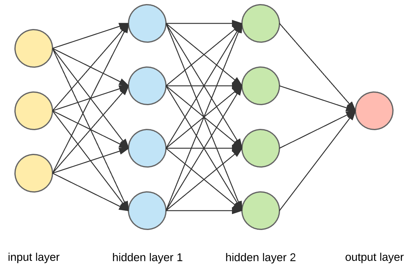
Consider an MLP with N layers, in each layer we are presented with M inputs. We are multiplying these with weights \(w_{ij}\) where i is the layer number while \(j\) is the neuron index in the layer. The output size of the layer will be the same as the neuron count in that layer. The feed-forward step for a densely connected neural network in each layer is pretty obvious:

# Python

def forward_pass(self, input_value):
    """
        Multiplying by W and adding b then applying the activation.
    """
    self.input = input_value
    self.activation_input = np.matmul(self.input, self.weights.T) + self.biases
    self.output = self.activation_fn.call(self.activation_input)
    return self.output

// C++

arma::Mat<double> DenseLayer::feedForward(const arma::Mat<double> &inputValue) {
    this->input = inputValue;
    this->activationInputs = this->input * this->weights + this->biases.t();
    this->output = this->activationFunction->call(this->activationInputs);
    return this->output;
}

In words, the input vector is multiplied by the weight matrix which is sized based on input size and output size provided. A bias vector is added to te result and thus we get the activation. We should add a non-linear activation function at the end of the layer since the chain of linear operations could be simplified into one linear operation. This way in each layer weights and biases are updated in each round and activation functions are applied. Moving on tu the back-propagation algorithm we need the derivative of weights and biases in each layer if the input is fixed on start. (Note: remember, in the post about neural style transfer, we actually modified one of the inputs and applied gradients on that.)

Another important step is weight initialization, since with not proper weights the network won’t learn properly with our optimization algorithm. Read more about weight initialization here.

# Python

def __init__(self, input_size, layer_size, activation_fn):
    self.input_size = input_size
    scaler = np.sqrt(2./(self.input_size + layer_size))
    self.weights = np.random.normal(size=(layer_size, input_size)) * scaler
    self.biases = np.random.normal(size=layer_size) * scaler
    self.activation_fn = activation_fn

// C++

DenseLayer::DenseLayer(unsigned int inputSize, unsigned int units,
                       std::string activationName) : inputSize(inputSize), units(units) {
    arma::arma_rng::set_seed(100); // for testing
    this->weights = arma::randn(inputSize, units) * sqrt(2. / (double) (inputSize + units));
    this->biases = arma::randn(units) * sqrt(2. / (double) (inputSize + units));
    /*
    * Some lines were intentionally left out.
    */
}

Back-propagation

Imagining the network as a chain/graph of operations we can easilly use the derivation rule of the composition. On the output of the network we have an objective, for classifiers the goal is to approximate the labels of inputs correctly. We define a loss for this that takes the actual label of the provided inputs and the approximated label. By the approximated label the loss function is a function of all the weights and baises of the network. If we call the output of the network \(\hat{z}\) and the loss is \(L\Big(\vec{z}, \hat{z}, \Big(\hat{W}_{i}, b_{i}\Big)_{i=1}^{layers}\Big)\) taking the derivative according to \(\vec{x}\) (the input) can be written as:

From this formula it can be seen that that each derivative can be calculated layer-wise with only the input from the layer preceeding it in the back-propagation process.

Therefore, for calculating the gradients we need to pass back the gradient of each layer through the network and multiply it with the gradient calculated in that layer.

Since we are interested mostly in gradients of weights and biases since we are going to update those via gradient descent:

Where it is easy to calculate the last term in the layer:

Doing the same for the bias vectors:

# Python
    def backprop(self, previous_gradient):
        self.activation_derivative = self.activation_fn.derivative(self.activation_input) # f'(Wx + b)
        self.intermediate_gradient = np.multiply(previous_gradient, self.activation_derivative) # f'(Wx + b) * received_grad -> recursive gradient flow
        self.bias_derivative = self.intermediate_gradient # df/db = f'(Wx + b) * 1
        self.weights_derivative = np.outer(self.intermediate_gradient, self.input) # f'(Wx + b) * x
        self.gradient = np.matmul(self.intermediate_gradient, self.weights)
        return self.gradient

// C++

arma::Mat<double> DenseLayer::backProp(arma::Mat<double> &previous_gradient) {
    this->activationDerivative = this->activationFunction->derivative(this->activationInputs);
    this->intermediateGradient = previous_gradient % this->activationDerivative.t();
    this->weightsGradient = this->intermediateGradient * this->input;
    return this->weights * this->intermediateGradient;
}

With this, we can implement almost every detail. The DenseLayer is therefore properly defined but we still need to create a model that loops through all layers, defines a loss and feeds the model with inputs while performing SGD as well.

Using MSE loss for simplicity:

# Python

def fit(self, x, y, lr=0.001, EPOCHS=5):
    for epoch in range(EPOCHS):
        for ind in range(x.shape[0]):
            yhat = self._forward_pass(x[ind])
            loss = np.sum((y[ind] - yhat)**2)
            grad = -2*(y[ind] - yhat)
            grad = self._backward_pass(grad)
            self._apply_grads(lr)
        if epoch % 5 == 0: print('Loss in epoch %d : %.5f' % (epoch, loss))

// C++

void Model::fit(const arma::mat &data, const arma::mat &target, double learningRate, int EPOCHS) {
    for (int i = 0; i < EPOCHS; ++i) {
        for (int row_ind = 0; row_ind < data.n_rows; ++row_ind) {
            arma::Mat<double> output = this->fullForwardPass(data.submat(row_ind, 0, row_ind, data.n_cols - 1));
            arma::mat gradient = this->fullBackwardPass(-2 * (target.at(row_ind) / 10. - output)); // percentages

            if (row_ind % 100 == 0) {
                std::cout << "Loss : " << arma::accu(arma::square(output - target.at(row_ind) / 10.)) << "\tEPOCH : "
                          << i + 1 << " " << row_ind
                          << "\tGradient size : " << arma::accu(arma::sqrt((arma::square(gradient)))) << std::endl;
            }

            this->applyGradients(learningRate);
        }
    }
}

The C++ code is not that readable since I had to hack it together to work properly. It is obvious from both of them that batching is not implemented and that after a full forward and backward pass gradients are applied with a learning rate set at the main program files before running the programs. In each layer gradients are applied to weights and biases:

# Python

def apply_gradients(self, lr):
        self.weights -= lr*self.weights_derivative
        self.biases -= lr*self.bias_derivative

// C++

void DenseLayer::applyGrads(double learningRate) {
    this->weights -= learningRate * this->weightsGradient.t();
    this->biases -= learningRate * this->intermediateGradient;
}

I have not mentioned yet how we calculate derivates. The easiest way is to predefine functions that we calculate analytically and they have call(value) and derivate(value) methods as well. A prime example of this is the implementation of the rectified linear unit:

# Python

class Relu:
    def call(self, x):
        return np.maximum(np.zeros(x.shape[0]), x)

    def derivative(self, x):
        return np.array([0 if val < 0 else 1 for val in x])

// C++

arma::Mat<double> ReLU::call(arma::Mat<double> value) {
    return arma::clamp(value, 0., arma::abs(value).max());
}

arma::Mat<double> ReLU::derivative(arma::Mat<double> value) {
    return arma::clamp(arma::sign(value), 0., 1.);
}

Just to showcase how models are defined, I used a Keras-like approach due to the clean interface it provides and the ease-of-use.

# Python

seq = Model()
seq.add(DenseLayer(784, 512, Relu()))
seq.add(DenseLayer(512, 256, Relu()))
seq.add(DenseLayer(256, 64, Relu()))
seq.add(DenseLayer(64, 1, Relu()))

seq.fit(x, y, lr=5e-6, EPOCHS=25)

// C++

Model model;
model.add(DenseLayer(784, 500, "relu"));
model.add(DenseLayer(500, 300, "relu"));
model.add(DenseLayer(300, 200, "relu"));
model.add(DenseLayer(200, 100, "relu"));
model.add(DenseLayer(100, 1, "sigmoid"));

model.fit(data, labels, 1e-1, 100);

I hope I could help however read this to understand back-propagation and densely connected neural network architecture. It was a shock to me how similiar the implementations actually were and that Python’s NumPy package is so optimized that the Python code actually run at comparable speeds to the C++ code. (It is mostly due to NumPy being compiled and C and provided as an API.)

@Regards, Alex

Alex Olar

Christian, foodie, physicist, tech enthusiast

Tweet Share