Visualizing the loss landscape

Visualizing the loss landscape

When evaluating the neural network we evaulate the same objective function used during training. For a classification task the most widely used loss function is the categorical cross-entropy which takes as input the one-hot probability distribution of the true image label as well as the prediction over the classes given by the deep neural network. We can state the the loss function is parametrized by the input dataset, the true labels and the learnt weights of the network:

Where y(x) is the one-hot distribution for the appropiate class of the sample x. What’s there to visualize on the loss? It is a function of the dataset we evaluate it on and the model’s parameters. The loss surface can be defined with respect to the model parameters. As modern convolutional networks can have millions (way more in some cases) of parameters a multitude of ways have been developed to use them to visualize the loss surface in lower dimensions. The paper Visualizing the Loss Landscape of Neural Nets proposes a solution of visualizing the loss surface with respec to modifying the weights of the underlying neural net in random, normalized directions.

Where \(\boldsymbol{\gamma}, \boldsymbol{\eta}\) are random directions in the vector space of the model weights. This method made it possible to parametrize the surface with \(\alpha, \beta\) parameters and therefore we can calculate its values alongside a 2D grid.

The idea of random directions for visualizing high-dimensional functions was not new but did not work for others beforehand. It is largely due to the fact that previously no one used filterwise normalization on the random directions. As CNNs are not parametrized by independent random variables but are highly structured into convolutional, densely connected parts each filter perturbation should therefore be perturbed on the scale of that learned filter.

Where j is the index of the filter and i is the index inside that flattened filter and d is the random direction we sampled from a pre-defined distribution (random normal).

Basically this is the theory. Sample to, independent random dierections in the same vector space as the weights and scale them filter-by-filter to amount for the different processing units and learnt filter scales. This method ensures that every part of the network is ‘properly’ perturbed and we can evaluate the f function on a grid of \(\alpha, \beta\) values and the given dataset.

Code

In order to experiments with different architectures we would need to pre-train all of them on the training set (ImageNet in this case) and evaluate them on the test set with the random directions alongside a grid to visualize their loss surface. PyTorch contains a few ImageNet-pretrained models that can be used in this scenario, so the training part could be skipped whilst the evaluation was done on the ImageNetV2 dataset since the original ImageNet data is not publicly available anymore and even tough I asked for access, it takes them a lot of time to provide it.

Loading the models is fairly easy:

import torch

model_ids = ['mobilenet_v2', 'vgg11', 'vgg11_bn', 'alexnet', 'vgg16', 'vgg16_bn', 'resnet18',
             'densenet161', 'inception_v3',
             'googlenet', 'resnext50_32x4d', 'mnasnet1_0',
             'resnet50']


def load_model(model_identifier):
    return torch.hub.load('pytorch/vision:v0.6.0', model_identifier, pretrained=True, verbose=False).eval()

Here I defined all available identifiers from the pytorch/vision:v0.6.0 GitHub respository and loaded them with the pre-trained weights and set them to evaluation mode.

Moving on comes the random direction generation and the filter perturbation part. Given a model -> torch.nn.Module it is possible to go through its named parameters:

def init_directions(model):
    noises = []

    n_params = 0
    for name, param in model.named_parameters():
        delta = torch.normal(.0, 1., size=param.size())
        nu = torch.normal(.0, 1., size=param.size())

        param_norm = torch.norm(param)
        delta_norm = torch.norm(delta)
        nu_norm = torch.norm(nu)

        delta /= delta_norm
        delta *= param_norm

        nu /= nu_norm
        nu *= param_norm

        noises.append((delta, nu))

        n_params += np.prod(param.size())

    print(f'A total of {n_params:,} parameters.')

    return noises

Above I calcualted the norm of both random vecotrs (in the flattented shape of the each filter) as well as the norm of the filter and collected the values into a noise list. This way if I loop over the named parameters again, I could easilly add/substract from the current value.

Basically that is the way I’ll initialize the network, in each grid point, in order to calculate the loss value with those parameters:

def init_network(model, all_noises, alpha, beta):
    with torch.no_grad():
        for param, noises in zip(model.parameters(), all_noises):
            delta, nu = noises
            # the scaled noises added to the current filter
            new_value = param + alpha * delta + beta * nu
            param.copy_(new_value)
    return model

Pretty much, that is it. Knowing all this we must pause for a while and consider the running time of this algorithm. Evaluating any function on a grid scales quadratically with the resolution we wish to achieve. Our loss function on the other hand also takes time to evaluate that scales linearly with the test dataset size. We need to run our network in each grid point N times to get the loss on the test dataset. With a large enough GPU we could fit enourmous batches into memory and the latter problem is solved, however, the former is the actual issue here. For high-precision visualization a resolution of 25 in each dimension (from -1 to 1) is not a lot, but already takes 625 full loss calculations. The visualizations on losslandscape.com must have taken days to render properly if not more.

Putting it all together

To be clear, the loss surface depends on the batch size chosen, the test dataset (obviously) and the noise selected. Given all that the actual loop that calcualtes the surface value (loss) in each grid point is the following:

# Creating the initial noise directions
noises = init_directions(load_model(model_id))

# Our loss function (for categorical problems)
crit = torch.nn.CrossEntropyLoss()

# The mesh-grid
A, B = np.meshgrid(np.linspace(-1, 1, RESOLUTION),
                   np.linspace(-1, 1, RESOLUTION), indexing='ij')

loss_surface = np.empty_like(A)

for i in range(RESOLUTION):
    for j in range(RESOLUTION):
        total_loss = 0.
        n_batch = 0
        alpha = A[i, j]
        beta = B[i, j]
        # Initilazing the network to the current directions (alpha, beta)
        net = init_network(load_model(model_id), noises, alpha, beta).to('cuda')
        for images, labels in dataloader:
            images = batch.to('cuda')
            labels = labels.to('cuda')
            # We do not net to acquire gradients
            with torch.no_grad():
                preds = net(images)
                loss = crit(preds, labels)
                total_loss += loss.item()
                n_batch += 1
        loss_surface[i, j] = total_loss / (n_batch * BATCH_SIZE)
        # Freeing up GPU memory
        del net
        torch.cuda.empty_cache()

All that remains is the visualizations. I have put all the code to my GitLab repository. The visualizations were initalially as simple as doing a contour plot on the grid but it turned out that for some networks, the loss rapidly went up, therefore I needed to log scale the surface in order to see it properly. Given all this, here are some pretty cool, moving 3D visualizations created by myself.

VGG16	VGG16-bn

VGG11	VGG11-bn

InceptionV3	Resnet18

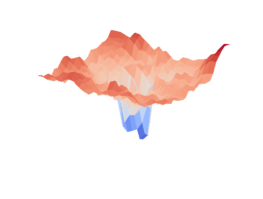
And the most amazing looking one, turned out to be mobilenet_v2:

MobileNetV2

We can clearly see that networks that include batch normalization have a very smooth loss surface while the initial VGG11/16 architectures not even have a clear minimum but they posess multiple minima when optimized.

Some experiments are still running, the repository will be updated.

Conclusion

It has been a while since I’ve written anything, I missed it tremendously but I had a lot to do at university, work and in life. I hope to be writing again soon, I have some ideas that might be useful to others as well. I already have a tool available for FROC curve generation. :)

References

• Visualizing the Loss Landscape of Neural Nets
• losslandscape.com
• original code of the paper authors
• my implementation discussed here

@Regards, Alex

Alex Olar

Christian, foodie, physicist, tech enthusiast

Tweet Share