Capsule Networks - a 'new' way of thinking
- 18 minsCapsule networks - a ‘new’ way of thinking
Capsule networks are building the essential blocks of image understanding as part of their optimization strategy. They are not hugely popular currently and by no means new but intuitively they make the most sense compared to wide-spread deep learning. As far as I know, Hinton originally came up with the idea more than twenty years ago but so far due to computational limitations and possibly many other factors I refer to as tricks, it could not have been properly achieved. Here, in this post, I’ll give a brief introduction to the basics and implement the algorithm in PyTorch alongside the MultiMNIST dataset, however, you can read the original paper as well.
What is a capsule network?
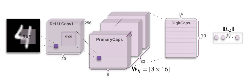
I already mentioned that this might be the most intuitive idea of how a human brain might process visual information. Capsules are the basic objects of visual perception. Such as in graphics we can build a scene hierarchically out of triangles, rectangles to the combinations of these and up to actual objects. Capsules capture this idea, they are vectors, representing very basic objects in the first ‘layer’ up to very complex objects, built up hierarchically from simpler ones. As we want to develop an algorithm that does this inversely, from pictures, we call this type of problem inverse graphics.
Let’s first build up an intuition about the most basic capsules. They can represent objects as simple triangles, or a 90-degree curve, a circle, etc. - we might want their length to represent the probability whether the object they represent is present in the current image or not. In the paper they apply a non-linear squashing operation they shrinks long-vectors to close to length 1, and small vectors close to length 0:
\[\vec{v} = \frac{||\vec{s}||^{2}}{1 + ||\vec{s}||^{2}} \cdot \frac{\vec{s}}{||\vec{s}||}\]Why do we use vectors, one might ask. Not only can their length represent the probability of presence but also, the values inside them can represent basic information about the color, line-width, zig-zagyness of the basic objects. Therefore, a capsule is way more intuitive than a simple neuron with a scalar value.
How is hierarchy built?
The tricky part is the hierarchy. We would like to achieve hierarchical dependency between certain capsules in consecutive layers. Only certain as not every basic object takes part in representing more complex objects. Let’s take a step back and just think about the basic objects representing ‘higher-order’ ones. Basic blocks need to be transformed into properly aligned shapes to form those complex blocks (e.g. house = rectangle + triangle in the right orientation). Vectors are manipulated via linear operations - matrix multiplication - so we need to learn those transformation matrices from lth layer capsules to l+1th layer capsules, between each consecutive capsule layer. The algorithm that helps to learn these weights and creates a hierarchy between capsules is called dynamic routing:
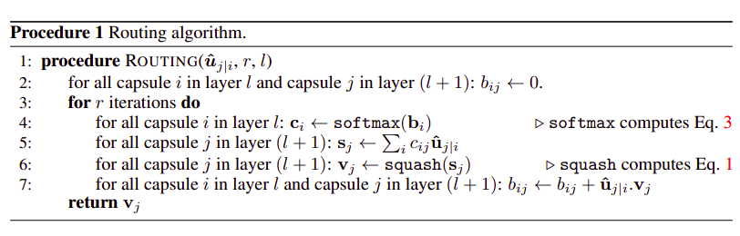
Here vectors u represent the capsules from the lth layer multiplied by the transformation weights between the lth and l+1th layers.
\[\hat{u}_{j | i} = \sum_{i}W_{ij}u_{i}\]Also, bs are the pre-softmax agreement scores that are initialized to 0 before dynamic routing and updated according to the agreement. What do they mean by agreement? The b scores initially after softmax would mean that the output of the l+1th layer v would be the squashed mean of all the transformed capsules from the l th layer (line 4-5-6. of the algorithm at the first iteration) - as the softmax of a uniform vector is filled with the length inverse in each position. However, by agreement, we want to measure how well the transformed first layer capsules u align with this output - leading to the agreement when the transformed original capsule and the current output point in the same direction. Capturing this cosine-similarity in the pre-softmax b weight we run through the routing iteration again and again (lines 4-7 in the procedure) finally leading to a hierarchical agreement between consecutive layers of capsules. In practice, 2-5 iterations are enough.
Finally, the classification task is achieved with a margin loss measuring the existence probability of the output vector v for each capsule, leading to multi-label classification.
\[L_{k} = T_{k}max(0, m^{+} - ||\vec{v}^{(k)}||)^{2} + \lambda (1 - T_{k}) max(0, ||\vec{v}^{(k)}|| - m^{-})^{2}\]Where T is an indicator function present at training time, indicating whether a possible class is present or not. While ms represent the negative and positive margins for desired (non-)existence.
All this in code
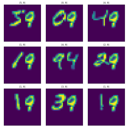
Capsule networks beat SOTA in multiple, overlapping MNIST digit classification. This also proves empirically that they built-up a notion of underlying, defining parts of an image.
MultiMNIST dataset
MNIST is available in basically all modern deep learning framework. To build a stochastically changing MultiMNIST dataset we need to load it first and randomly select two digits from different classes, then apply augmentations and return them with the corresponding labels in a single binary vector.
from PIL import Image
import numpy as np
import torch
import torchvision

class MultiMnist(torch.utils.data.Dataset):
    """
     Code left out to make this section shorter.
    """

    def __getitem__(self, index):
        index1 = index
        index2 = random.randint(0, len(self) - 1)

        image1, label1 = self.mnist[index1]
        image2, label2 = self.mnist[index2]

        while label1 == label2:
            index2 = random.randint(0, len(self) - 1)
            image2, label2 = self.mnist[index2]

        if self.image_transforms:
            image1 = self.image_transforms(image1)
            image2 = self.image_transforms(image2)

        x = np.array(image1)
        y = np.array(image2)
        blend = np.where(x > y, x, y)
        image = Image.fromarray(blend)

        if self.transforms:
            image = self.transforms(image)

        label = np.zeros(shape=(1, 10), dtype=np.float32)
        label[:, label1] = 1
        label[:, label2] = 1

        if self.target_transform:
            label = self.target_transform(label)

        return image, label
Basically the only tricky part here is the way we blend the two image tensors together:
x = np.array(image1)
y = np.array(image2)
blend = np.where(x > y, x, y)
image = Image.fromarray(blend)
This method resulted in the best visual results for me, so I went on with this type of blending, however, you’d find a different solution for RGB inputs.
In the GitHub repository of the code I also added some code to be able to make the batching process deterministic for testing purposes. This was also the first Python project in which I experimented with proper testing and GitHub CI jobs.
The capsule network
The squashing must be computationally safe, therefore the \(\epsilon\) tricks in the norm:
def _squash(self, tensor, axis=-1, epsilon=1e-8):
    norm = self._norm(tensor, axis=axis, keepdims=True)
    squash = T.square(norm) / (1. + T.square(norm))
    unit = tensor / norm
    return unit * squash

def _norm(self, tensor, axis=-1, keepdims=False, epsilon=1e-8):
    squared_norm = T.sum(T.square(tensor), axis=axis, keepdims=keepdims)
    return T.sqrt(squared_norm + epsilon)
So far this has been pretty straight-forward, moving on to the initialization of the network:
import torch as T
import torch.nn.functional as F
from torch.nn import Conv2d


class CapsuleNetwork(T.nn.Module):
    def __init__(self, batch_size, capsule_dims=[8, 16], n_caps=[1152, 10]):
        super(CapsuleNetwork, self).__init__()
        self.capsule_dims = capsule_dims
        self.n_caps = n_caps
        self.conv1 = Conv2d(in_channels=1,
                            out_channels=256,
                            kernel_size=9,
                            stride=1)
        self.conv2 = Conv2d(in_channels=256,
                            out_channels=256,
                            kernel_size=9,
                            stride=2)

        stddev = .01
        self.transformation_weights = T.nn.Parameter(T.normal(
            mean=0,
            std=stddev,
            size=(1, n_caps[0], n_caps[1], capsule_dims[1], capsule_dims[0])),
            requires_grad=True)

        self.raw_scores = T.nn.Parameter(
            T.zeros(size=(batch_size, self.n_caps[0], self.n_caps[1], 1, 1)))
My implementation is closely based on that of Aurélion Géron’s from this notebook and presentation where the hyperparameters have been precisely calculated for a (28, 28) input size. The main takeaways here are the following:
-
We need to initialize the set of transformation weight between the first and last capsule layers (yes, this is a 2-layer capsule net, and is already computationally heavy)
-
We also need to initialize the raw scores that will be used to calculate the softmax [without requiring the gradients since this parameter is not going to be optimized]
The network otherwise uses convolutional blocks for initial feature extraction to form the basic capsules.
The forward pass
def forward(self, inputs):
    x, y = inputs

    x = F.relu(self.conv1(x))
    x = F.relu(self.conv2(x))

    batch_size, channels, width, heigth = x.shape

    n_first_layer_capsules = width * height * channels // self.capsule_dims[0]

    first_layer_capsule_dim = self.capsule_dims[0]

    x = T.reshape(x, (batch_size, n_first_layer_capsules, first_layer_capsule_dim))

    x = self._squash(x)

    x = x.view(batch_size, self.n_caps[0], 1, self.capsule_dims[0],
                1).repeat(1, 1, self.n_caps[1], 1, 1)

    tiled_transformation_weights = self.transformation_weights.repeat(
        batch_size, 1, 1, 1, 1)

    routing_weights = F.softmax(self.raw_weights, dim=2)

    caps2 = T.matmul(tiled_transformation_weights, x)
    weighted_preds = T.mul(routing_weights, caps2)
    weighted_sum = T.sum(weighted_preds, axis=1, keepdims=True)
    caps2_round1 = self._squash(weighted_sum, axis=-2)

    caps2_round1_tiled = caps2_round1.repeat(1, self.n_caps[0], 1, 1, 1)

    agreement = T.matmul(caps2.transpose(3, 4), caps2_round1_tiled)
    raw_weights_2 = T.add(self.raw_weights, agreement)
    routing_weights = F.softmax(raw_weights_2, dim=2)

    weighted_preds = T.mul(routing_weights, caps2)
    weighted_sum = T.sum(weighted_preds, axis=1, keepdims=True)
    caps2_round2 = self._squash(weighted_sum, axis=-2)

    caps2_round2_tiled = caps2_round2.repeat(1, self.n_caps[0], 1, 1, 1)

    agreement = T.matmul(caps2.transpose(3, 4), caps2_round2_tiled)
    raw_weights_3 = T.add(self.raw_weights, agreement)
    routing_weights = F.softmax(raw_weights_3, dim=2)

    weighted_preds = T.mul(routing_weights, caps2)
    weighted_sum = T.sum(weighted_preds, axis=1, keepdims=True)
    caps2_round3 = self._squash(weighted_sum, axis=-2)

    caps2 = caps2_round3.squeeze()

    caps2_normed = self._norm(caps2)
    preds = T.argmax(caps2_normed, axis=-1).squeeze()

    return preds, caps2, caps2_normed
Here the first step is to extract features with the convolutional blocks from the image and then resize it to (batch_size, n_first_layer_capsules, first_layer_capsule_dim) then squash it alongside the n_first_layer_capsules dimension. After squashing we expand its dimensionality alongside the selected axis and repeat it n_second_layer_capsules time to be able to calculate the transformation weight between each pair in the first and second/last capsule layer - the transformation weight should be the same for each element of the batch hence the tiling. Afterward, the initial routing scores are calculated from the raw, zeroed-out scores.
# Steps in the forward pass 2.
# ...

x = x.view(batch_size, self.n_caps[0], 1, self.capsule_dims[0],
            1).repeat(1, 1, self.n_caps[1], 1, 1)

tiled_transformation_weights = self.transformation_weights.repeat(
    batch_size, 1, 1, 1, 1)

routing_scores = F.softmax(self.raw_scores, dim=2)
Moving on we can implement the dynamic routing steps, not in a loop, but the old-fashioned (and very lazy) way of writing out each iteration:
# Steps in the forward pass 3.
# ...

caps2 = T.matmul(tiled_transformation_weights, x)
weighted_preds = T.mul(routing_weights, caps2)
weighted_sum = T.sum(weighted_preds, axis=1, keepdims=True)
caps2_round1 = self._squash(weighted_sum, axis=-2)

caps2_round1_tiled = caps2_round1.repeat(1, self.n_caps[0], 1, 1, 1)

agreement = T.matmul(caps2.transpose(3, 4), caps2_round1_tiled)
raw_weights_2 = T.add(self.raw_weights, agreement)
routing_weights = F.softmax(raw_weights_2, dim=2)

weighted_preds = T.mul(routing_weights, caps2)
weighted_sum = T.sum(weighted_preds, axis=1, keepdims=True)
caps2_round2 = self._squash(weighted_sum, axis=-2)

caps2_round2_tiled = caps2_round2.repeat(1, self.n_caps[0], 1, 1, 1)

agreement = T.matmul(caps2.transpose(3, 4), caps2_round2_tiled)
raw_weights_3 = T.add(self.raw_weights, agreement)
routing_weights = F.softmax(raw_weights_3, dim=2)

weighted_preds = T.mul(routing_weights, caps2)
weighted_sum = T.sum(weighted_preds, axis=1, keepdims=True)
caps2_round3 = self._squash(weighted_sum, axis=-2)

caps2 = caps2_round3.squeeze()

caps2_normed = self._norm(caps2)
preds = T.argmax(caps2_normed, axis=-1).squeeze()

return preds, caps2, caps2_normed
These steps are the lines 4-7. in the algorithm block repeated 3 times. In the end, the last capsules are normed and many ‘views’ are returned.
The loss
The loss calculation is exactly the same as the equation written out above but in code looks the following:
def margin_loss(outputs, one_hot_labels):
    margin_positive = .9
    margin_negative = .1
    lambd = .5

    batch_size, _ = one_hot_labels.shape

    postive_loss = torch.square(
        torch.max(torch.zeros_like(outputs), margin_positive - outputs))
    negative_loss = torch.square(
        torch.max(torch.zeros_like(outputs), outputs - margin_negative))

    negative_loss = torch.mul((1. - one_hot_labels), negative_loss)
    postive_loss = torch.mul(one_hot_labels, postive_loss)

    loss = postive_loss + lambd * negative_loss

    return torch.sum(loss) / batch_size
During training the margin loss looks the following way:
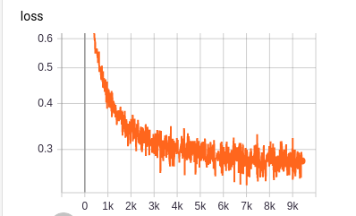
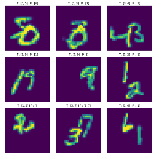
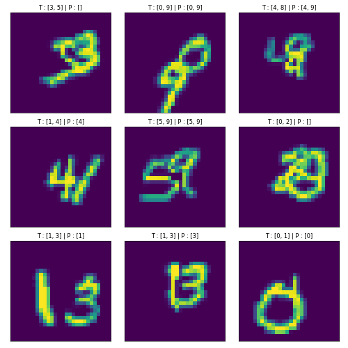
And the network produces sometimes correct predictions for the overlapping, MultiMNIST inputs (examples):
Conclusion
Well, I am especially proud of this post and I had tried to do my best explaining the architecture and the algorithm in my terms for others to understand. Hope you come back. :)
References
@Regards, Alex

Alex Olar
Christian, foodie, physicist, tech enthusiast