Glia cell detection using FAIR's Detectron2 framework
- 10 minsReview
I have written about glial cell detection in June. Since than a lot has happened and I’ve been busy with other projects and tasks in research but in my spare time I experimented with Detectron2.
I think I also mentioned previously that nat all neurons are annotated which is a huge issue when dealing with false positive rates since the 50% rate is misleading.
Detectron2
Basically FAIR developed a new framework for object recognition and segmentation with Detectron2. Now you don’t have to modify your own fork of Detectron and include your dataset and update config files. Everything happens programmatically. The basics steps are:
- set up Detectron2 preferably in a
condaenvironment since probably very few people have clean base environments on their computers - convert your data to COCO format and such as:
- where
neuron_2019_<train/test/validation/all>contains images corresponding to training, testing, validation (and all images just for convenience)
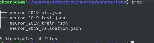
- where
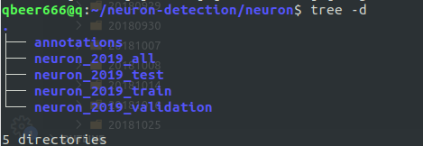
- annotations are in COCO format, stored in JSON for training, testing, validation (and all)
- with Detectron2 you just need to register the dataset!
An this last one is the important part. Previously a lot of set up was needed and training was a pain as it was only possible to follow it through ugly JSON formatted outputs during training epochs.
Know visualizations are integrated, tensorboard is integrated and training can be followed.
Data handling remained the same, luckily. The COCO format can be described as follows:
def create_coco_json(self, output_name):
        self._build_images()
        self._build_annotations()
        coco_output = {
            "info": self.info,
            "licenses": self.licenses,
            "categories": self.categories,
            "images": self.images,
            "annotations": self.annotations
        }
Where the self.categories is a list of dictionaries with the desired categories and the background:
self.categories = [{
            "supercategory": "neuron",
            "id": 1,
            "name": "neuron"
        }, {
            "supercategory": "background",
            "id": 2,
            "name": "background"
        }]  # pseude-class with no instances for TRAINING
While the images, annotations are defined as:
image = {
                "license": 1,
                "file_name": patch_name,
                "coco_url": "",
                "height": 500,
                "width": 500,
                "date_captured": str(datetime.datetime.now()),
                "flickr_url": "",
                "id": patch_id
}

anno = {
    # (x0, y0),
    # (x1, y0),
    # (x1, y1),
    # (x0, y1)
    "segmentation": [[neuron_annotation[0], neuron_annotation[1],
                        neuron_annotation[0] + \
                        neuron_annotation[2], neuron_annotation[1],
                        neuron_annotation[0] + \
                        neuron_annotation[2], neuron_annotation[1] + \
                        neuron_annotation[3],
                        neuron_annotation[0], neuron_annotation[1] + neuron_annotation[3]]],
    "area": neuron_annotation[2] * neuron_annotation[3],
    "iscrowd": 0,
    "image_id": patch["id"],
    "bbox": neuron_annotation.tolist(),
    "category_id": 1,
    "id": annotation_id
}
This structure is straight-forward although there are some changes in Detectron2 since segmentations are given back as RLE (run-length encoded) strings. I have used Detectron for bounding box detection so this is not a necessity for me.
Training setup
This is the technical part, if the reader is not interested this is the part to skip.
Registering your dataset:
register_coco_instances("neuron_2019_train", {}, "./neuron/annotations/neuron_2019_train.json",
                        "./neuron/neuron_2019_train/")

register_coco_instances("neuron_2019_test", {}, "./neuron/annotations/neuron_2019_test.json",
                        "./neuron/neuron_2019_test/")
Basic configuration is also available in the Colab notebook provided by FAIR:
cfg = get_cfg()
cfg.merge_from_file(
    "../detectron2/configs/COCO-InstanceSegmentation/mask_rcnn_R_50_FPN_3x.yaml")
cfg.DATASETS.TRAIN = ("neuron_2019_test",)
cfg.DATASETS.TEST = ()
cfg.DATALOADER.NUM_WORKERS = 2
# initialize from model zoo
cfg.MODEL.WEIGHTS = "detectron2://COCO-InstanceSegmentation/mask_rcnn_R_50_FPN_3x/137849600/model_final_f10217.pkl"
cfg.SOLVER.IMS_PER_BATCH = 5
cfg.SOLVER.BASE_LR = 0.0025
# 300 iterations seems good enough, but you can certainly train longer
cfg.SOLVER.MAX_ITER = 1000
# faster, and good enough for this toy dataset
cfg.MODEL.ROI_HEADS.BATCH_SIZE_PER_IMAGE = 128
cfg.MODEL.ROI_HEADS.NUM_CLASSES = 1  # glial cell
cfg.OUTPUT_DIR = './detectron2_results/'
Here we use a pre-trained mask_rcnn model and a very small learning rate and 1 class for detectron to predict for ROIs.
For testing trained model weights are loaded back and a predictor is run on the dataset. The dataset can be sampled and bbox metadata can be acquired by default as well as a visualizer:
cfg.MODEL.WEIGHTS = os.path.join(cfg.OUTPUT_DIR, "model_final.pth")
# set the testing threshold for this model
cfg.MODEL.ROI_HEADS.SCORE_THRESH_TEST = 0.7
cfg.DATASETS.TEST = ("neuron_2019_test", )
predictor = DefaultPredictor(cfg)

evaluator = COCOEvaluator("neuron_2019_test", cfg,
                          False, output_dir=cfg.OUTPUT_DIR)
val_loader = build_detection_test_loader(cfg, "neuron_2019_test")
inference_on_dataset(trainer.model, val_loader, evaluator)

dataset_dicts = get_detection_dataset_dicts(["neuron_2019_test"])
metadata = MetadataCatalog.get("neuron_2019_test")
ind = 0
for d in random.sample(dataset_dicts, 3):
    im = cv2.imread(d["file_name"])
    outputs = predictor(im)
    v = Visualizer(im[:, :, ::-1],
                   metadata=metadata,
                   scale=0.8,
                   instance_mode=ColorMode.IMAGE_BW   # remove the colors of unsegmented pixels
                   )
    v = v.draw_instance_predictions(outputs["instances"].to("cpu"))
    cv2.imwrite("./detectron2_results/test_viz_%d.jpg" % ind, v.get_image()[:, :, ::-1])
    ind += 1
Results
Given the dataset I updated my code to run with Detectron2. Visualizations through Tensorboard are possible and extremely useful:
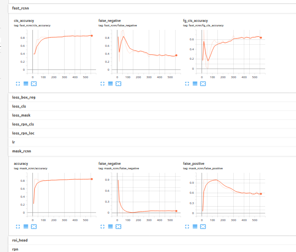
Since the neuron dataset which actually contains glial cells contains cells and not natural images pre-trained weights help but the model needs some time to get good results and converge. I gave it 1000 iteration just to make sure it’s working. What you can see here is the middle of the training basically.
COCO metrics are the following for the separated test set:
Running per image evaluation...
Evaluate annotation type *bbox*
DONE (t=8.43s).
Accumulating evaluation results...
DONE (t=0.13s).
 Average Precision  (AP) @[ IoU=0.50:0.95 | area=   all | maxDets=100 ] = 0.205
 Average Precision  (AP) @[ IoU=0.50      | area=   all | maxDets=100 ] = 0.649
 Average Precision  (AP) @[ IoU=0.75      | area=   all | maxDets=100 ] = 0.043
 Average Precision  (AP) @[ IoU=0.50:0.95 | area= small | maxDets=100 ] = 0.205
 Average Precision  (AP) @[ IoU=0.50:0.95 | area=medium | maxDets=100 ] = -1.000
 Average Precision  (AP) @[ IoU=0.50:0.95 | area= large | maxDets=100 ] = -1.000
 Average Recall     (AR) @[ IoU=0.50:0.95 | area=   all | maxDets=  1 ] = 0.028
 Average Recall     (AR) @[ IoU=0.50:0.95 | area=   all | maxDets= 10 ] = 0.213
 Average Recall     (AR) @[ IoU=0.50:0.95 | area=   all | maxDets=100 ] = 0.299
 Average Recall     (AR) @[ IoU=0.50:0.95 | area= small | maxDets=100 ] = 0.299
 Average Recall     (AR) @[ IoU=0.50:0.95 | area=medium | maxDets=100 ] = -1.000
 Average Recall     (AR) @[ IoU=0.50:0.95 | area= large | maxDets=100 ] = -1.000
Since we are interested in bbox predictions we can see that the results are not very good but promising. For glial cell detection we don’t need high IoU and average between 0.5-0.65 is well enough and it that range we can already achieved over 60% average precision. Recall should also improve in that range but we can’t see that. Luckily I have modified that COCO evaluation code to include the desired ranges, so:
Running per image evaluation...
Evaluate annotation type *bbox*
DONE (t=0.87s).
Accumulating evaluation results...
DONE (t=0.03s).
 *Average Precision  (AP) @[ IoU=0.50:0.65 | area=   all | maxDets= 50 ] = 0.466
 *Average Precision  (AP) @[ IoU=0.50      | area=   all | maxDets= 50 ] = 0.646
 Average Precision  (AP) @[ IoU=0.65      | area=   all | maxDets= 50 ] = 0.262
 Average Recall     (AR) @[ IoU=0.50:0.65 | area=   all | maxDets=  5 ] = 0.249
 Average Recall     (AR) @[ IoU=0.50:0.65 | area=   all | maxDets= 10 ] = 0.429
 *Average Recall     (AR) @[ IoU=0.50:0.65 | area=   all | maxDets= 50 ] = 0.602
With only 1000 iterations we have achieved < 60% recall and precision score!
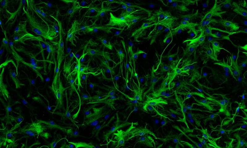
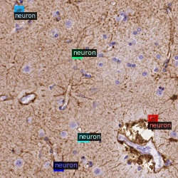
Some results:
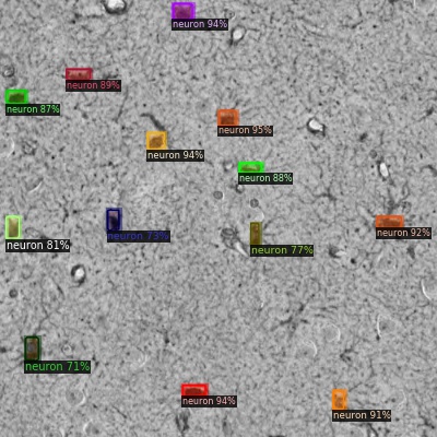
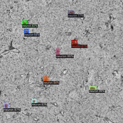
The images are visualized with Detectron2 since such cool tools are included.
Merry Christmas to you all and a Happy New Year!
@Regards, Alex

Alex Olar
Christian, foodie, physicist, tech enthusiast